splicelogic: differential transcripts to splice events
Beatriz Campillo
Michael I. Love
07/27/2026
Source:vignettes/splicelogic.Rmd
splicelogic.RmdIntroduction
splicelogic allows users to find alternative splicing events after performing differential transcript usage (DTU) analysis. Unlike event-based tools that work at the junction level, splicelogic operates on whole transcript structures: each transcript and all its exons are annotated with a DTU effect estimate, allowing splicing events to be derived directly from transcript quantification with full isoform context. By comparing up- and down-regulated transcripts, splicelogic can detect skipped exons, included exons, mutually exclusive exons, retained introns, and alternative 5’ and 3’ splice sites. Because it takes transcript-level effect estimates as input, it is compatible with any upstream DTU method (including DRIMSeq, DEXSeq, satuRn, and edgeR), supporting flexible experimental designs.
splicelogic operates on exon-level data stored as GRanges objects. Given a set of exons annotated with a coefficient column indicating differential transcript usage (DTU), splicelogic identifies the following types of splicing events:
- Skipped exons (SE) – exons skipped in up-regulated transcripts
- Included exons (IE) – exons included in up-regulated transcripts
- Mutually exclusive exons (MXE) – pairs of exons where one is included and another is excluded in up-regulated transcripts compared to down-regulated transcripts
- Retained introns (RI) – intronic regions that are retained as part of an exon in up-regulated transcripts
- Alternative 5’ (A5SS) – exons in up-regulated transcripts that share the same 3’ splice site but differ at the 5’ splice site from exons in down-regulated transcripts
- Alternative 3’ (A3SS) – as above, but differing in the 3’ splice site
These are detected using a series of functions,
e.g. find_se(), find_ie(), etc. described
below.
Related methods
Several tools exist for detecting alternative splicing from RNA-seq data and analyzing its consequences.
IsoformSwitchAnalyzeR — a comprehensive workflow that performs DTU testing, annotates the resulting isoform switches with splicing event types, and predicts functional consequences such as domain loss and NMD.
GeneStructureTools — takes differential splicing results from read-based tools such as Whippet or leafcutter (which detect splicing events from junction counts), classifies the event types, and assesses their structural and functional consequences such as ORF changes, NMD potential, and UTR structure.
isoformic — a visualization and functional interpretation pipeline for pre-computed differential transcript expression results. It organizes transcripts by biotype (protein-coding, lncRNA, NMD, etc.) and provides expression profile plots and functional enrichment analysis.
splicelogic differs in its main input and focus: it does not perform DTU testing, and also does not take pre-computed splicing events as input. Instead, it takes transcript-level DTU results (effect estimates and adjusted p-values from any upstream method) already mapped onto exon structures, and directly classifies the type of splicing event from the comparison of up- and down-regulated isoforms.
By operating on exon-level GRanges with attached DTU statistics, splicelogic provides a flexible framework for users to identify and interpret splicing events in the context of their specific experimental design and choice of DTU method. GRanges are a common data structure in Bioconductor for representing genomic features such as exons and introns, making splicelogic compatible with a wide range of already available tools and existing workflows. For example, it can be combined with plyranges for dplyr-like operations on exons/introns following identification of regulated exon and introns, and Biostrings for extraction of sequence surrounding splice events.
Quick start
With DTU results attached to a GRanges of the exons from significant transcripts, one can use the following code to identify splice events:
Input data
splicelogic assumes the user has run a differential transcript usage (DTU) or differential splicing analysis providing 1) a statistic for defining a set of significant transcripts, e.g. adjusted p-value and 2) an effect estimate with direction, e.g. GLM estimated coefficient or change in percent-spliced-in (PSI), see upstream methods.
It also assumes the user has information about the genomic ranges for the exons of each transcript. splicelogic provides a set of helper functions for generating these exon ranges, see obtaining exon ranges. One helper function can simply take a partition of the transcripts as input (if no DTU analysis was performed upstream).
The exons should be provided in a flat GRanges
object (one range per exon), containing exon-level metadata in
mcols(exons) such as the gene ID, transcript ID, rank in
the transcript, and the estimated change or at least direction of change
from the differential analysis. Again, this object can be compiled by
splicelogic helper functions described below.
Required columns for exons:
| Column | Description |
|---|---|
gene_id |
Gene identifier |
tx_id |
Transcript identifier |
exon_rank |
Exon rank within the transcript |
coef_col = "<user supplied>" |
differential effect estimate for the transcript |
The differential effect estimate column is specified by the user in
preprocess(). This should be the differential effect
estimate associated with the specific transcript containing the exon,
and minimally could indicate the direction of effect with
+1/-1. Positive values indicate up-regulated exons and
negative values indicate down-regulated exons. All exons from the same
transcript will share the same value for this column.
Output format
All find_*() functions return a GRanges whose
ranges are the exons detected to be involved in an event. Each row
therefore carries the user’s original exon-level metadata — including
tx_id, the transcript that the detected exon belongs to —
together with the following event-specific columns added in
mcols() that describe the paired transcript
against which the event is defined:
| Column | Description |
|---|---|
event_type |
Type of splicing event detected ("se",
"ie", "mxe", "ri",
"a5ss", or "a3ss"). |
event_tx_id |
Transcript ID of the paired transcript that, together with
the detected exon’s transcript (tx_id), defines the
event. |
event_estimate |
DTU coefficient (estimate) of the paired
transcript. |
event_<col> |
One column per name in metadata(gr)$additional_columns,
prefixed with event_, carrying the corresponding value from
the paired transcript. |
In short: the original metadata columns describe the transcript that
contains the returned exon, while all columns with the prefix
event_* describe the paired transcript against which the
event is defined.
Jones et al mouse long read dataset
For demonstration, we will use a published mouse long read dataset and its reported splicing changes.
The citation is:
Emma F. Jones, Timothy C. Howton, Victoria L. Flanary, Amanda D. Clark, Brittany N. Lasseigne Long-read RNA sequencing identifies region- and sex-specific C57BL/6J mouse brain mRNA isoform expression and usage Mol Brain 17, 40 (2024). doi: 10.1186/s13041-024-01112-7
Information about the paper, including code and publicly available data can be found at this URL:
https://github.com/lasseignelab/230227_EJ_MouseBrainIsoDiv
In the abstract, Jones et al. describe the experiment:
To assess differences in AS across the cerebellum, cortex, hippocampus, and striatum by sex, we generated and analyzed Oxford Nanopore Technologies (ONT) long-read RNA sequencing (lrRNA-Seq) C57BL/6J mouse brain cDNA libraries. From > 85 million reads that passed quality control metrics, we calculated differential gene expression (DGE), differential transcript expression (DTE), and differential transcript usage (DTU) across brain regions and by sex.
Here we will focus on the cortex-specific sex comparison, comparing
female to male mice. For demonstration in the vignette, we have saved a
small subset of the results from this Zenodo entry. The dataset
was made available under an MIT license. For information on how the DTU
table was saved, this is noted in inst/scripts/make-data.R.
Generating the exons BED file is also described there, which was
downloaded and parsed from the GENCODE M31 GTF file (comprehensive gene
annotation). See below for more details on how to prepare exons for use
with splicelogic.
Loading example data
In this section we load the small example dataset that has been prepared for this vignette. Note that in a typical splicelogic workflow, the exons GRanges would be loaded from a TxDb. See the obtaining exon ranges section below for further details.
We load the differential transcript usage analysis from the Jones et al. paper. Specifically, we load the transcripts found to exhibit DTU in the F vs M comparison in cortex.
The DTU table for this example, and the exons for the differential
transcripts have been saved in the extdata directory of
splicelogic.
The DTU table was generated by the authors of Jones et al., which used IsoformSwitchAnalyzeR to process DTU analysis results from DEXSeq, running on transcript counts instead of exon counts. For splicelogic, we only require that some statistical method was used to test DTU, that we have adjusted p-values allowing us to subset to an FDR bounded set, and that we have a numeric value indicating the direction of change associated with each transcript.
library(readr)
# load DTU results
dir <- system.file("extdata", package="splicelogic")
dtu_table <- readr::read_delim(file.path(dir, "dtu_table.tsv"))
We load from BED file the 601 exons from GENCODE M31 annotation for the 49 differential transcripts, and attach the metadata columns.
library(plyranges)
exons_file <- "exons_M31.bed.gz"
exons_mcols_file <- "exons_mcols.tsv.gz"
exons <- plyranges::read_bed(file.path(dir, exons_file))
mcols(exons) <- DataFrame(
  readr::read_delim(file.path(dir, exons_mcols_file))
)
Finally, we add Seqinfo for mm49, the reference mouse
genome for GENCODE M31.
Next, we join the DTU results onto the exons GRanges.
This is necessary for the splicelogic functions to know which
transcripts are up- or down-regulated, and to which gene the exons and
transcripts belong.
The code below matches the transcript IDs in the exons
metadata with the DTU results table, and then binds the two tables
before assigning back to exons.
txp_idx <- match(exons$tx_id, dtu_table$tx_id)
cols_to_add <- dtu_table[txp_idx, ] |> dplyr::select(-tx_id)
merged_DF <- S4Vectors::cbind(mcols(exons), cols_to_add)
mcols(exons) <- merged_DF
As of Bioc 3.23 and plyranges version 1.32, the above code to add metadata columns from an additional table can be replaced with the following:
exons <- exons |>
  plyranges::join_mcols_left(dtu_table, by = "tx_id")
splicelogic is designed to take as input the exons from significantly changed transcripts, so we first filter out transcripts that were not signficant at FDR 10%.
## GRanges object with 2 ranges and 8 metadata columns:
##       seqnames            ranges strand |   exon_id            exon_name
##          <Rle>         <IRanges>  <Rle> | <numeric>          <character>
##   [1]    chr10 88036955-88037154      + |    304310 ENSMUSE00000574345.8
##   [2]    chr10 88037674-88037772      + |    304316 ENSMUSE00000417972.4
##       exon_rank                 tx_id               gene_id   gene_name
##       <numeric>           <character>           <character> <character>
##   [1]         1 ENSMUST00000020248.16 ENSMUSG00000020056.17      Washc3
##   [2]         2 ENSMUST00000020248.16 ENSMUSG00000020056.17      Washc3
##        estimate      padj
##       <numeric> <numeric>
##   [1] -0.264716 0.0449634
##   [2] -0.264716 0.0449634
##   -------
##   seqinfo: 61 sequences (1 circular) from mm39 genome
Finding splicing events
Preprocessing input data
The first step is to run preprocess(), which prepares
the exons for event detection. This function checks the
input data, ensures that the necessary columns are present:
library(splicelogic)
sig_exons <- sig_exons |>
  preprocess(coef_col = "estimate")
sig_exons |> head(2)
## GRanges object with 2 ranges and 11 metadata columns:
## seqnames ranges strand | exon_id exon_name
## <Rle> <IRanges> <Rle> | <numeric> <character>
## [1] chr10 88036955-88037154 + | 304310 ENSMUSE00000574345.8
## [2] chr10 88037674-88037772 + | 304316 ENSMUSE00000417972.4
## exon_rank tx_id gene_id gene_name
## <numeric> <character> <character> <character>
## [1] 1 ENSMUST00000020248.16 ENSMUSG00000020056.17 Washc3
## [2] 2 ENSMUST00000020248.16 ENSMUSG00000020056.17 Washc3
## estimate padj key nexons internal
## <numeric> <numeric> <character> <integer> <logical>
## [1] -0.264716 0.0449634 ENSMUST00000020248.1.. 7 FALSE
## [2] -0.264716 0.0449634 ENSMUST00000020248.1.. 7 TRUE
## -------
## seqinfo: 61 sequences (1 circular) from mm39 genomepreprocess() also accepts an optional
additional_columns argument. This lets us specify which
metadata columns we want to bring over from the paired transcript
(event_tx_id) into the event output. It takes a character
vector of column names already present in mcols(exons);
each will then appear in the output as event_<col>.
See ?preprocess for details.
Finding individual events
Next we can run the various functions for calculating different types of splicing events.
Skipped exons (SE)
For example, we can calculate exons that are skipped in up-regulated transcripts relative to down-regulated transcripts, across all genes. As these are skipped in the up-regulated transcripts, it is expected that the exons returned belong to down-regulated transcripts:
skipped <- sig_exons |> find_se()
skipped
## GRanges object with 1 range and 11 metadata columns:
## seqnames ranges strand | exon_id exon_name
## <Rle> <IRanges> <Rle> | <numeric> <character>
## [1] chr17 66647479-66647535 - | 480827 ENSMUSE00000443570.7
## exon_rank tx_id gene_id gene_name
## <numeric> <character> <character> <character>
## [1] 14 ENSMUST00000097291.10 ENSMUSG00000052105.18 Mtcl1
## estimate padj event_type event_tx_id event_estimate
## <numeric> <numeric> <character> <character> <numeric>
## [1] -2.9732 0.00970121 se ENSMUST00000086693.12 2.88524
## -------
## seqinfo: 61 sequences (1 circular) from mm39 genomeIncluded exons (IE)
included <- sig_exons |> find_ie()
included
## GRanges object with 3 ranges and 11 metadata columns:
## seqnames ranges strand | exon_id exon_name
## <Rle> <IRanges> <Rle> | <numeric> <character>
## [1] chr14 20517526-20517591 - | 408079 ENSMUSE00001423050.2
## [2] chr1 163739641-163739706 + | 12966 ENSMUSE00000368805.4
## [3] chr8 120884207-120884236 + | 250989 ENSMUSE00001243257.2
## exon_rank tx_id gene_id gene_name
## <numeric> <character> <character> <character>
## [1] 6 ENSMUST00000100844.6 ENSMUSG00000021814.18 Anxa7
## [2] 20 ENSMUST00000077642.12 ENSMUSG00000026585.14 Kifap3
## [3] 10 ENSMUST00000034281.13 ENSMUSG00000031824.16 6430548M08Rik
## estimate padj event_type event_tx_id event_estimate
## <numeric> <numeric> <character> <character> <numeric>
## [1] 3.02406 0.018472554 ie ENSMUST00000065504.17 -3.34894
## [2] 1.04389 0.010395185 ie ENSMUST00000027877.7 -1.70708
## [3] 4.14230 0.000995041 ie ENSMUST00000108951.8 -3.42759
## -------
## seqinfo: 61 sequences (1 circular) from mm39 genomeMutually exclusive exons (MXE)
mx <- sig_exons |> find_mxe()
mx
## GRanges object with 2 ranges and 11 metadata columns:
## seqnames ranges strand | exon_id exon_name
## <Rle> <IRanges> <Rle> | <numeric> <character>
## [1] chr12 91799829-91799996 - | 374021 ENSMUSE00001304078.2
## [2] chr12 91798541-91798558 - | 374018 ENSMUSE00001473756.2
## exon_rank tx_id gene_id gene_name
## <numeric> <character> <character> <character>
## [1] 4 ENSMUST00000021347.12 ENSMUSG00000020964.15 Sel1l
## [2] 4 ENSMUST00000178462.8 ENSMUSG00000020964.15 Sel1l
## estimate padj event_type event_tx_id event_estimate
## <numeric> <numeric> <character> <character> <numeric>
## [1] -3.28535 0.00171934 mxe ENSMUST00000178462.8 2.99384
## [2] 2.99384 0.00171934 mxe ENSMUST00000021347.12 -3.28535
## -------
## seqinfo: 61 sequences (1 circular) from mm39 genomeRetained introns (RI)
Here we do not find retained introns, and the function returns an empty vector.
ri <- sig_exons |> find_ri()
ri
## GRanges object with 0 ranges and 0 metadata columns:
## seqnames ranges strand
## <Rle> <IRanges> <Rle>
## -------
## seqinfo: no sequencesAlternative 5’ and 3’ splice sites (A5/3SS)
a5ss <- sig_exons |> find_a5ss()
a5ss
## GRanges object with 5 ranges and 11 metadata columns:
## seqnames ranges strand | exon_id exon_name
## <Rle> <IRanges> <Rle> | <numeric> <character>
## [1] chr10 88081618-88081868 + | 304334 ENSMUSE00001310024.2
## [2] chr14 20529963-20530189 - | 408097 ENSMUSE00000901772.3
## [3] chr8 120887954-120892045 + | 250998 ENSMUSE00000446870.6
## [4] chr9 21858242-21858348 + | 266133 ENSMUSE00001322549.2
## [5] chr9 21858900-21860203 + | 266139 ENSMUSE00001327764.2
## exon_rank tx_id gene_id gene_name
## <numeric> <character> <character> <character>
## [1] 7 ENSMUST00000182183.8 ENSMUSG00000020056.17 Washc3
## [2] 1 ENSMUST00000100844.6 ENSMUSG00000021814.18 Anxa7
## [3] 13 ENSMUST00000034281.13 ENSMUSG00000031824.16 6430548M08Rik
## [4] 7 ENSMUST00000190387.7 ENSMUSG00000040563.14 Plppr2
## [5] 9 ENSMUST00000190387.7 ENSMUSG00000040563.14 Plppr2
## estimate padj event_type event_tx_id event_estimate
## <numeric> <numeric> <character> <character> <numeric>
## [1] 9.19059 0.086737576 a5ss ENSMUST00000020248.16 -0.264716
## [2] 3.02406 0.018472554 a5ss ENSMUST00000065504.17 -3.348940
## [3] 4.14230 0.000995041 a5ss ENSMUST00000108951.8 -3.427593
## [4] 6.33671 0.006078234 a5ss ENSMUST00000046371.13 -0.694010
## [5] 6.33671 0.006078234 a5ss ENSMUST00000046371.13 -0.694010
## -------
## seqinfo: 61 sequences (1 circular) from mm39 genome
a3ss <- sig_exons |> find_a3ss()
a3ss
## GRanges object with 9 ranges and 11 metadata columns:
## seqnames ranges strand | exon_id exon_name
## <Rle> <IRanges> <Rle> | <numeric> <character>
## [1] chr10 88037014-88037154 + | 304312 ENSMUSE00001309977.2
## [2] chr10 88055115-88055222 + | 304327 ENSMUSE00001223513.2
## [3] chr14 20505329-20506669 - | 408059 ENSMUSE00000564348.6
## [4] chr8 120840891-120841056 + | 250964 ENSMUSE00000678589.2
## [5] chr8 112437109-112438026 - | 262490 ENSMUSE00001391518.2
## [6] chr4 101504990-101505022 + | 107521 ENSMUSE00000631777.3
## [7] chr4 101513375-101513492 + | 107524 ENSMUSE00000671573.2
## [8] chr9 21849570-21849860 + | 266124 ENSMUSE00001334761.2
## [9] chr17 66643977-66645149 - | 480823 ENSMUSE00000791759.2
## exon_rank tx_id gene_id gene_name
## <numeric> <character> <character> <character>
## [1] 1 ENSMUST00000182183.8 ENSMUSG00000020056.17 Washc3
## [2] 5 ENSMUST00000182183.8 ENSMUSG00000020056.17 Washc3
## [3] 14 ENSMUST00000100844.6 ENSMUSG00000021814.18 Anxa7
## [4] 1 ENSMUST00000034281.13 ENSMUSG00000031824.16 6430548M08Rik
## [5] 7 ENSMUST00000212349.2 ENSMUSG00000031955.11 Bcar1
## [6] 1 ENSMUST00000106927.2 ENSMUSG00000035212.15 Leprot
## [7] 3 ENSMUST00000106927.2 ENSMUSG00000035212.15 Leprot
## [8] 1 ENSMUST00000190387.7 ENSMUSG00000040563.14 Plppr2
## [9] 14 ENSMUST00000086693.12 ENSMUSG00000052105.18 Mtcl1
## estimate padj event_type event_tx_id event_estimate
## <numeric> <numeric> <character> <character> <numeric>
## [1] 9.19059 0.086737576 a3ss ENSMUST00000020248.16 -0.264716
## [2] 9.19059 0.086737576 a3ss ENSMUST00000020248.16 -0.264716
## [3] 3.02406 0.018472554 a3ss ENSMUST00000065504.17 -3.348940
## [4] 4.14230 0.000995041 a3ss ENSMUST00000108951.8 -3.427593
## [5] 3.85659 0.027009405 a3ss ENSMUST00000166232.4 -3.477749
## [6] 9.13055 0.018472554 a3ss ENSMUST00000030254.15 -2.405394
## [7] 9.13055 0.018472554 a3ss ENSMUST00000030254.15 -2.405394
## [8] 6.33671 0.006078234 a3ss ENSMUST00000046371.13 -0.694010
## [9] 2.88524 0.013967132 a3ss ENSMUST00000097291.10 -2.973204
## -------
## seqinfo: 61 sequences (1 circular) from mm39 genomeFinding all events
The following function wraps the above ones to find all events.
all_events <- sig_exons |> find_all_events()## Calculating skipped exon events...## Calculating included exon events...## Calculating mutually exclusive exon events...## Calculating retained intron events...## Calculating alternative 5' splice site events...## Calculating alternative 3' splice site events...## Done! 20 events detected.
all_events## GRanges object with 20 ranges and 11 metadata columns:
## seqnames ranges strand | exon_id exon_name
## <Rle> <IRanges> <Rle> | <numeric> <character>
## [1] chr17 66647479-66647535 - | 480827 ENSMUSE00000443570.7
## [2] chr14 20517526-20517591 - | 408079 ENSMUSE00001423050.2
## [3] chr1 163739641-163739706 + | 12966 ENSMUSE00000368805.4
## [4] chr8 120884207-120884236 + | 250989 ENSMUSE00001243257.2
## [5] chr12 91799829-91799996 - | 374021 ENSMUSE00001304078.2
## ... ... ... ... . ... ...
## [16] chr8 112437109-112438026 - | 262490 ENSMUSE00001391518.2
## [17] chr4 101504990-101505022 + | 107521 ENSMUSE00000631777.3
## [18] chr4 101513375-101513492 + | 107524 ENSMUSE00000671573.2
## [19] chr9 21849570-21849860 + | 266124 ENSMUSE00001334761.2
## [20] chr17 66643977-66645149 - | 480823 ENSMUSE00000791759.2
## exon_rank tx_id gene_id gene_name
## <numeric> <character> <character> <character>
## [1] 14 ENSMUST00000097291.10 ENSMUSG00000052105.18 Mtcl1
## [2] 6 ENSMUST00000100844.6 ENSMUSG00000021814.18 Anxa7
## [3] 20 ENSMUST00000077642.12 ENSMUSG00000026585.14 Kifap3
## [4] 10 ENSMUST00000034281.13 ENSMUSG00000031824.16 6430548M08Rik
## [5] 4 ENSMUST00000021347.12 ENSMUSG00000020964.15 Sel1l
## ... ... ... ... ...
## [16] 7 ENSMUST00000212349.2 ENSMUSG00000031955.11 Bcar1
## [17] 1 ENSMUST00000106927.2 ENSMUSG00000035212.15 Leprot
## [18] 3 ENSMUST00000106927.2 ENSMUSG00000035212.15 Leprot
## [19] 1 ENSMUST00000190387.7 ENSMUSG00000040563.14 Plppr2
## [20] 14 ENSMUST00000086693.12 ENSMUSG00000052105.18 Mtcl1
## estimate padj event_type event_tx_id event_estimate
## <numeric> <numeric> <character> <character> <numeric>
## [1] -2.97320 0.009701213 se ENSMUST00000086693.12 2.88524
## [2] 3.02406 0.018472554 ie ENSMUST00000065504.17 -3.34894
## [3] 1.04389 0.010395185 ie ENSMUST00000027877.7 -1.70708
## [4] 4.14230 0.000995041 ie ENSMUST00000108951.8 -3.42759
## [5] -3.28535 0.001719345 mxe ENSMUST00000178462.8 2.99384
## ... ... ... ... ... ...
## [16] 3.85659 0.02700941 a3ss ENSMUST00000166232.4 -3.47775
## [17] 9.13055 0.01847255 a3ss ENSMUST00000030254.15 -2.40539
## [18] 9.13055 0.01847255 a3ss ENSMUST00000030254.15 -2.40539
## [19] 6.33671 0.00607823 a3ss ENSMUST00000046371.13 -0.69401
## [20] 2.88524 0.01396713 a3ss ENSMUST00000097291.10 -2.97320
## -------
## seqinfo: 61 sequences (1 circular) from mm39 genome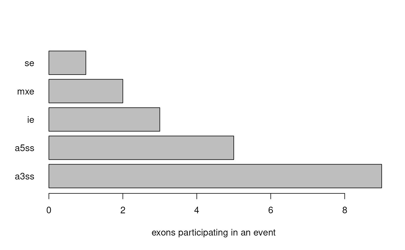
Upstream methods
splicelogic is designed to operate downstream of differential transcript usage (DTU). DTU methods test whether the relative proportions of transcripts within a gene differ between experimental conditions.
In general, any upstream method that produces transcript-resolved differential usage statistics can be used with splicelogic, provided that results include:
- a per-transcript directional effect estimate (e.g. a model
coefficient, change in isoform fraction, deltaPSI, etc.), and
- an adjusted p-value (or equivalent significance metric by thresholding).
Common upstream methods include:
satuRn — fits quasi-binomial generalized linear models to transcript usage proportions and performs scalable transcript-level DTU testing. Particularly well suited to larger datasets. Gene-level testing recommended via stageR.
DRIMSeq — models transcript proportions within genes using a Dirichlet-Multinomial framework, with both gene-level and transcript-level testing.
BANDITS — a Bayesian hierarchical DTU method that models transcript usage using a Dirichlet-Multinomial and explicitly accounts for mapping uncertainty using equivalence classes, with both gene-level and transcript-level testing.
DEXSeq — primarily a differential exon usage (DEU) method based on negative binomial GLMs, but commonly used in transcript-level DTU workflows (e.g. the rnaseqDTU Bioconductor 2018 workflow). The log2 fold change coefficients from DEXSeq can be used directly with splicelogic.
limma and edgeR (
diffSplice/diffSpliceDGE) — can be used for DTU analyses (as well as exon-level), with both gene-level and transcript-level testing.
Regardless of which method is used, the per-transcript DTU statistics
(effect estimates and adjusted p-values) have to be mapped onto the
individual exons of each transcript to produce an exon-level
GRanges (see Obtaining exon
ranges). This annotated GRanges is the starting point for
splicelogic, beginning with preprocess() and then
followed by event-specific functions (find_se(),
find_ie(), etc.).
Obtaining exon ranges
Using prepare_exons()
prepare_exons() extracts exon ranges from a
TxDb object and merges them with your DTU results table. It
returns a flat GRanges ready for preprocess() and
the find_* functions. Typical usage shown in the following
code:
We demonstrate using GENCODE v32 (human genes). The first step is to
load a TxDb object. Typically, a user would supply their own
GTF to txdbmaker::makeTxDbFromGFF() to generate this. For
this demonstration we will load a pre-constructed TxDb from
Bioconductor’s AnnotationHub.
suppressPackageStartupMessages({
  library(AnnotationHub)
  library(AnnotationDbi)
  library(GenomicFeatures)
})
ah <- AnnotationHub()
txdb <- ah[["AH75191"]] # GENCODE v32 (human)
## loading from cache
suppressPackageStartupMessages({
  library(tibble)
})
txps <- txdb |>
  AnnotationDbi::select(
    keys(txdb, "TXID"), c("TXNAME","GENEID"), "TXID"
  ) |>
  tibble::as_tibble() |>
  dplyr::select(tx_num = TXID, tx_id = TXNAME, gene_id = GENEID) |>
  dplyr::filter(!is.na(gene_id))
## 'select()' returned 1:1 mapping between keys and columns
txps## # A tibble: 227,462 × 3
## tx_num tx_id gene_id
## <int> <chr> <chr>
## 1 1 ENST00000456328.2 ENSG00000223972.5
## 2 2 ENST00000450305.2 ENSG00000223972.5
## 3 3 ENST00000473358.1 ENSG00000243485.5
## 4 4 ENST00000469289.1 ENSG00000243485.5
## 5 5 ENST00000607096.1 ENSG00000284332.1
## 6 6 ENST00000606857.1 ENSG00000268020.3
## 7 7 ENST00000642116.1 ENSG00000240361.2
## 8 8 ENST00000492842.2 ENSG00000240361.2
## 9 9 ENST00000641515.2 ENSG00000186092.6
## 10 10 ENST00000335137.4 ENSG00000186092.6
## # ℹ 227,452 more rows
# simulate DTU results
sim_dtu_table <- txps |>
  dplyr::mutate(
    padj = runif(dplyr::n()),
    effect_est = rnorm(dplyr::n())
  )
sim_dtu_table
## # A tibble: 227,462 × 5
## tx_num tx_id gene_id padj effect_est
## <int> <chr> <chr> <dbl> <dbl>
## 1 1 ENST00000456328.2 ENSG00000223972.5 0.0808 -0.497
## 2 2 ENST00000450305.2 ENSG00000223972.5 0.834 0.938
## 3 3 ENST00000473358.1 ENSG00000243485.5 0.601 -1.84
## 4 4 ENST00000469289.1 ENSG00000243485.5 0.157 1.53
## 5 5 ENST00000607096.1 ENSG00000284332.1 0.00740 0.882
## 6 6 ENST00000606857.1 ENSG00000268020.3 0.466 -2.10
## 7 7 ENST00000642116.1 ENSG00000240361.2 0.498 -0.443
## 8 8 ENST00000492842.2 ENSG00000240361.2 0.290 -1.60
## 9 9 ENST00000641515.2 ENSG00000186092.6 0.733 -0.124
## 10 10 ENST00000335137.4 ENSG00000186092.6 0.773 -0.576
## # ℹ 227,452 more rowsWe now build the exons GRanges with
prepare_exons():
human_exons <- prepare_exons(
  txdb, sim_dtu_table, coef_col = "effect_est", verbose = TRUE
)
## Extracting exons from TxDb...## Mapping transcript IDs...## Merging DTU results onto exons...## Done. Returned 1372308 exon ranges from 227462 unique transcripts.
human_exons <- human_exons |>
  filter(padj < .01) |>
  preprocess(coef_col = "effect_est")
Comparing two sets
If one has two sets of transcripts to compare, for example, a set of
transcripts of interest versus a reference set, one can use
prepare_exons_by_partition() as an alternative entry point.
It accepts either two GRanges objects (each carrying
exon_rank, gene_id, and tx_id) or
two character vectors of transcript IDs (in which case a TxDb
must be supplied to look up exon coordinates). The two sets are passed
as the up and down arguments; internally the
function assigns estimate = +1 to the up set
and estimate = -1 to the down set, and returns
a combined GRanges ready to pass to preprocess()
with coef_col = "estimate". This route is useful for
comparing two transcript sets of interest directly, without needing
per-transcript effect estimates from a DTU analysis. See
?prepare_exons_by_partition for details.
Manual construction
This section walks through the steps that
prepare_exons() performs internally. This is useful if one
needs more control over the process or want to understand how exon
ranges are built from a TxDb.
The following extracts the exons grouped by transcript from the TxDb:
# extract exons as a GRangesList
exons_list <- GenomicFeatures::exonsBy(
  txdb,
  by="tx"
  )
# Our DTU table aligns with txps, which aligns with the names
# of the GRangesList. prepare_exons() handles alignment checks.
names(exons_list) <- sim_dtu_table$tx_id
Next, we flatten the exons:
flat_exons <- unlist(exons_list)
# swap tx_id with exon_name as the names of the GRanges
flat_exons$tx_id <- names(flat_exons) # store transcript ids
names(flat_exons) <- flat_exons$exon_name
Finally, we add the DTU results and gene ID:
Session info
## R version 4.5.2 (2025-10-31)
## Platform: x86_64-pc-linux-gnu
## Running under: Ubuntu 24.04.3 LTS
##
## Matrix products: default
## BLAS:   /usr/lib/x86_64-linux-gnu/openblas-pthread/libblas.so.3
## LAPACK: /usr/lib/x86_64-linux-gnu/openblas-pthread/libopenblasp-r0.3.26.so;  LAPACK version 3.12.0
##
## locale:
##  [1] LC_CTYPE=en_US.UTF-8       LC_NUMERIC=C
##  [3] LC_TIME=en_US.UTF-8        LC_COLLATE=en_US.UTF-8
##  [5] LC_MONETARY=en_US.UTF-8    LC_MESSAGES=en_US.UTF-8
##  [7] LC_PAPER=en_US.UTF-8       LC_NAME=C
##  [9] LC_ADDRESS=C               LC_TELEPHONE=C
## [11] LC_MEASUREMENT=en_US.UTF-8 LC_IDENTIFICATION=C
##
## time zone: UTC
## tzcode source: system (glibc)
##
## attached base packages:
## [1] stats4    stats     graphics  grDevices utils     datasets  methods
## [8] base
##
## other attached packages:
##  [1] tibble_3.3.1           GenomicFeatures_1.62.0 AnnotationDbi_1.72.0
##  [4] Biobase_2.70.0         AnnotationHub_4.0.0    BiocFileCache_3.0.0
##  [7] dbplyr_2.6.0           splicelogic_1.1.2      plyranges_1.30.1
## [10] dplyr_1.2.1            GenomicRanges_1.62.1   Seqinfo_1.0.0
## [13] IRanges_2.44.0         S4Vectors_0.48.1       BiocGenerics_0.56.0
## [16] generics_0.1.4         readr_2.2.0
##
## loaded via a namespace (and not attached):
##  [1] tidyselect_1.2.1            blob_1.3.0
##  [3] filelock_1.0.3              Biostrings_2.78.0
##  [5] bitops_1.0-9                fastmap_1.2.0
##  [7] RCurl_1.98-1.19             GenomicAlignments_1.46.0
##  [9] XML_3.99-0.23               digest_0.6.39
## [11] lifecycle_1.0.5             KEGGREST_1.50.0
## [13] RSQLite_3.53.3              magrittr_2.0.5
## [15] compiler_4.5.2              rlang_1.3.0
## [17] sass_0.4.10                 tools_4.5.2
## [19] utf8_1.2.6                  yaml_2.3.12
## [21] rtracklayer_1.70.1          knitr_1.51
## [23] S4Arrays_1.10.1             htmlwidgets_1.6.4
## [25] bit_4.6.0                   curl_7.1.0
## [27] DelayedArray_0.36.1         abind_1.4-8
## [29] BiocParallel_1.44.0         purrr_1.2.2
## [31] withr_3.0.3                 desc_1.4.3
## [33] grid_4.5.2                  SummarizedExperiment_1.40.0
## [35] cli_3.6.6                   rmarkdown_2.31
## [37] crayon_1.5.3                ragg_1.5.2
## [39] otel_0.2.0                  httr_1.4.8
## [41] tzdb_0.5.0                  rjson_0.2.23
## [43] DBI_1.3.0                   cachem_1.1.0
## [45] parallel_4.5.2              BiocManager_1.30.27
## [47] XVector_0.50.0              restfulr_0.0.17
## [49] matrixStats_1.5.0           vctrs_0.7.3
## [51] Matrix_1.7-6                jsonlite_2.0.0
## [53] hms_1.1.4                   bit64_4.8.2
## [55] systemfonts_1.3.2           jquerylib_0.1.4
## [57] glue_1.8.1                  pkgdown_2.2.1
## [59] codetools_0.2-20            BiocVersion_3.22.0
## [61] GenomeInfoDb_1.46.2         BiocIO_1.20.0
## [63] UCSC.utils_1.6.1            pillar_1.11.1
## [65] rappdirs_0.3.4              htmltools_0.5.9
## [67] R6_2.6.1                    httr2_1.3.0
## [69] textshaping_1.0.5           vroom_1.7.1
## [71] evaluate_1.0.5              lattice_0.22-9
## [73] png_0.1-9                   Rsamtools_2.26.0
## [75] cigarillo_1.0.0             memoise_2.0.1
## [77] bslib_0.11.0                SparseArray_1.10.10
## [79] xfun_0.60                   fs_2.1.0
## [81] MatrixGenerics_1.22.0       pkgconfig_2.0.3