SEESAW - Allelic expression analysis with Salmon and Swish
01/03/2025
allelic.RmdIntroduction
In this vignette, we describe usage of a suite of tools, SEESAW, Statistical Estimation of allelic Expression using Salmon and Swish, which allow for testing allelic imbalance across samples.
The methods are described in Wu et al. (2022) doi: 10.1101/2022.08.12.503785.
SEESAW makes use of Swish (Zhu et al. 2019) for paired inference, which is an extension of the SAMseq (Li and Tibshirani 2011) methods for permutation-based FDR control.
Quick start
Minimal code for running SEESAW is shown below.
On the command line:
# generate diploid txome with g2gtools:
# http://churchill-lab.github.io/g2gtools/
> salmon index -p #threads -t diploid_fasta -i diploid_txome --keepDuplicates
> salmon quant -i diploid_txome -l A -p #threads \
  --numBootstraps 30 -o output -1 read1 -2 read2
From within R/Bioconductor:
# first build tx2gene to gene- or TSS-level
# (for isoform level skip `tx2gene`)
library(ensembldb)
library(plyranges)
# gene level:
tx2gene <- transcripts(edb) %>%
  select(tx_id, group_id=gene_id)
# TSS level:
tx2gene <- makeTx2Tss(edb, maxgap=50) %>%
  select(tx_id, gene_id, group_id, tss)
# import counts:
y <- importAllelicCounts(
  coldata, a1="alt", a2="ref",
  format="wide", tx2gene=tx2gene
)
# testing with Swish:
y <- labelKeep(y)
y <- y[mcols(y)$keep,]
# see below for other tests and details
y <- swish(y, x="allele", pair="sample", fast=1)
mcols(y)$qvalue # <-- gives FDR-bounded sets
Method overview
Type of tests
SEESAW allows for testing global allelic imbalance across all samples (pairwise testing within each individual), as well as differential, or dynamic allelic imbalance (pairwise allelic fold changes estimated within individual, followed by testing across two groups, or along an additional covariate). Each of these allelic imbalance (AI) analyses takes into account the potentially heterogeneous amount of inferential uncertainty per sample, per feature (transcript, transcript-group, or gene), and per allele.
Steps in SEESAW
Running SEESAW involves generation of a diploid transcriptome
(e.g. using g2gtools,
construction of a diploid Salmon index (specifying
--keepDuplicates), followed by Salmon quantification with a
number of bootstrap
inferential replicates (we recommend 30 bootstrap replicates). These
three steps (diploid reference preparation, indexing, quantification
with bootstraps) provide the input data for the following statistical
analyses in R/Bioconductor. The steps shown in this vignette leverage
Bioconductor infrastructure including SummarizedExperiment for
storage of input data and results, tximport for data import,
and GRanges and Gviz for plotting.
In short the SEESAW steps are as listed, and diagrammed below:
- g2gtools (diploid reference preparation)
- Salmon indexing with
--keepDuplicates - Salmon quantification with bootstraps
-
makeTx2Tss()aggregates data to TSS-level (optional) -
importAllelicCounts()creates a SummarizedExperiment - Swish analysis:
labelKeep()andswish()(skip scaling) - Plotting
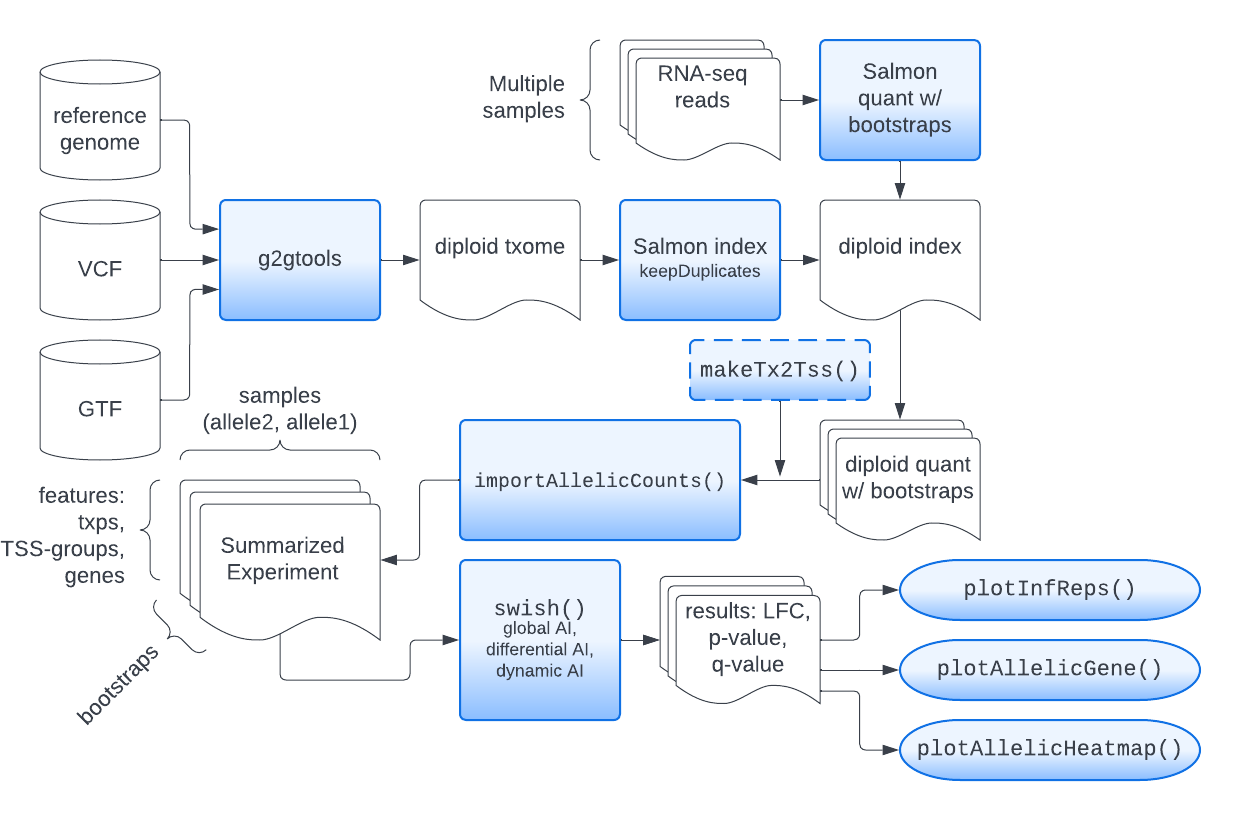
Below we demonstrate an analysis where transcripts are grouped by
their transcription start site (TSS), although gene-level or
transcript-level analysis is also possible. Additionally, any custom
grouping could be used, by manually generating a t2g table
as shown below. Special plotting functions in fishpond
facilitate visualization of allelic and isoform changes at different
resolutions, alongside gene models. In three examples, we perform global
AI testing, differential AI testing, and dynamic AI testing, in all
cases on simulated data associated with human genes.
Linking transcripts to TSS
We begin assuming steps 1-3 have been completed. We can use the
makeTx2Tss function to generate a GRanges object
t2g that connects transcripts to transcript groups.
suppressPackageStartupMessages(library(ensembldb))
library(EnsDb.Hsapiens.v86)
library(fishpond)
edb <- EnsDb.Hsapiens.v86
t2g <- makeTx2Tss(edb) # GRanges object
mcols(t2g)[,c("tx_id","group_id")]
## DataFrame with 216741 rows and 2 columns
## tx_id group_id
## <character> <character>
## ENST00000456328 ENST00000456328 ENSG00000223972-11869
## ENST00000450305 ENST00000450305 ENSG00000223972-12010
## ENST00000488147 ENST00000488147 ENSG00000227232-29570
## ENST00000619216 ENST00000619216 ENSG00000278267-17436
## ENST00000473358 ENST00000473358 ENSG00000243485-29554
## ... ... ...
## ENST00000420810 ENST00000420810 ENSG00000224240-2654..
## ENST00000456738 ENST00000456738 ENSG00000227629-2659..
## ENST00000435945 ENST00000435945 ENSG00000237917-2663..
## ENST00000435741 ENST00000435741 ENSG00000231514-2662..
## ENST00000431853 ENST00000431853 ENSG00000235857-5685..Alternatively for gene-level analysis, one could either prepare a
t2g data.frame with tx_id and
gene_id columns, or a t2g GRanges
object with a column group_id that is equal to
gene_id.
Importing allelic counts
Here we will use simulated data, but we can import allelic counts
with the importAllelicCounts() function. It is best to read
over the manual page for this function. For TSS-level analysis, the
t2g GRanges generated above should be passed to
the tx2gene argument. This will summarize transcript-level
counts to the TSS level, and will attach rowRanges that
provide the genomic locations of the grouped transcripts. Note that
importAllelicCounts does not yet have the ability to
automatically generate ranges based on sequence hashing (as occurs in
tximeta).
Filtering features
Because we use --keepDuplicates in the step when we
build the Salmon index, there will be a number of features in which
there is no information about the allelic expression in the reads. We
can find these features in bootstrap data by examining when the
inferential replicates are nearly identical for the two alleles, as this
is how the EM will split the reads. Removing these features avoids
downstream problems during differential testing. Code for this filtering
follows:
Global allelic imbalance
We begin by generating a simulated data object that resembles what
one would obtain with importAllelicCounts(). The import
function arranges the a2 (non-effect) allelic counts first,
followed by the a1 (effect) allelic counts. Allelic ratios
are calculated as a1/a2, which follows the notational
standard in PLINK and other tools.
set.seed(1)
y <- makeSimSwishData(allelic=TRUE)
colData(y)
## DataFrame with 20 rows and 2 columns
## allele sample
## <factor> <factor>
## s1-a2 a2 sample1
## s2-a2 a2 sample2
## s3-a2 a2 sample3
## s4-a2 a2 sample4
## s5-a2 a2 sample5
## ... ... ...
## s6-a1 a1 sample6
## s7-a1 a1 sample7
## s8-a1 a1 sample8
## s9-a1 a1 sample9
## s10-a1 a1 sample10
levels(y$allele) # a1/a2 allelic fold changes## [1] "a2" "a1"A hidden code chunk is used to add ranges from the EnsDb to
the simulated dataset. For a real dataset, the ranges would be added
either by importAllelicCounts (if using
tx2gene) or could be added manually for transcript- or
gene-level analysis, using the rowRanges<- setter
function. The ranges are only needed for the
plotAllelicGene plotting function below.
<hidden code chunk>We can already plot a heatmap of allelic ratios, before performing statistical testing. We can see in the first gene, ADSS, there appear to be two groups of transcripts with opposing allelic fold change. SEESAW makes use of pheatmap for plotting a heatmap of allelic ratios.
y <- computeInfRV(y) # for posterior mean, variance
gene <- rowRanges(y)$gene_id[1]
idx <- mcols(y)$gene_id == gene
plotAllelicHeatmap(y, idx=idx)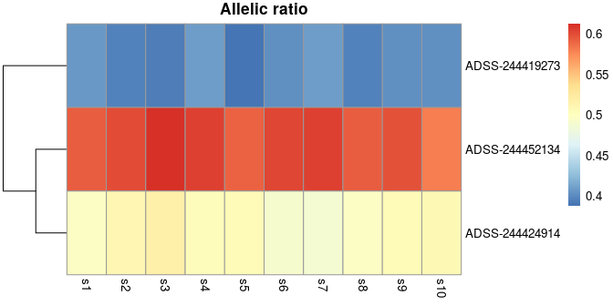
The following two functions perform a Swish analysis, comparing the allelic counts within sample, while accounting for uncertainty in the assignment of the reads. The underlying test statistic is a Wilcoxon signed-rank statistic, which compares the two allele counts from each sample, so a paired analysis.
Scaling: Note that we do not use
scaleInfReps in the allelic pipeline. Because we compare
the two alleles within samples, there is no need to perform scaling of
the counts to adjust for sequencing depth. We simply import counts,
filter low counts with lableKeep and then run the
statistical testing with swish.
Fast mode: for basic allelic analysis, we use a
paired test, comparing one allele to the other. The default in
swish for a simple paired test is to use a Wilcoxon signed
rank test statistic with bootstrap aggregation and permutation
significance. The ranks must be recomputed per permutation, which is a
slow operation that is not necessary with other designs in
swish. A faster test statistic is the one-sample z-score,
which gives similar results. Here we demonstrate using the fast version
of the paired test. Note that fast=1 is only relevant for
simple paired tests, not for other designs, which are already fast.
## Error in get(paste0(generic, ".", class), envir = get_method_env()) :
##   object 'type_sum.accel' not found
Plotting results
We can return to the heatmap, and now add q-values, etc. For details
on adding metadata to a pheatmap plot object, see
?pheatmap.
dat <- data.frame(minusLogQ=-log10(mcols(y)$qvalue[idx]),
                  row.names=rownames(y)[idx])
plotAllelicHeatmap(y, idx=idx, annotation_row=dat)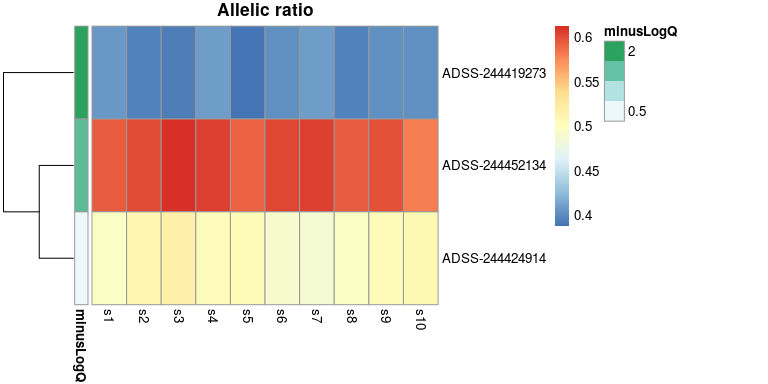
In order to visualize the inferential uncertainty, we can make use of
plotInfReps():
par(mfrow=c(2,1), mar=c(1,4.1,2,2))
plotInfReps(y, idx=1, x="allele", cov="sample", xaxis=FALSE, xlab="")
plotInfReps(y, idx=2, x="allele", cov="sample", xaxis=FALSE, xlab="")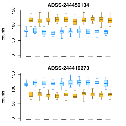
Plotting results in genomic context
For analysis at the isoform or TSS-level, it may be useful to display
results within a gene, relating the allelic differences to various gene
features. SEESAW provides plotAllelicGene() in order to
build visualization of Swish test statistics, allelic proportions, and
isoform proportions, in a genomic context, making use of Gviz.
Note that this function is not relevant for gene-level AI analysis. The
first three arguments to plotAllelicGene() are the
SummarizedExperiment object, the name of a gene (should match
gene_id column), and a TxDb or EnsDb to
use for plotting the gene model at the top. The statistics and
proportions are then plotted at the first position of the feature
(start for + features and end for
- features).
gene <- rowRanges(y)$gene_id[1]
plotAllelicGene(y, gene, edb, ideogram=FALSE)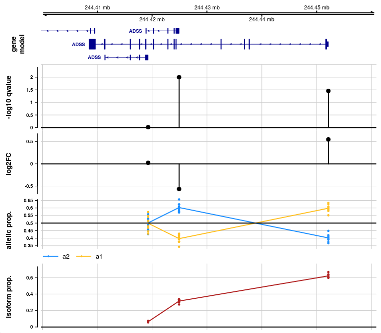
You can also specify the gene using symbol:
plotAllelicGene(y, symbol="ADSS", db=edb, ideogram=FALSE)
In the allelic proportion and isoform proportion tracks, a line is drawn through the mean proportion for a2 and a1 allele, and for the isoform proportion, across samples, at the start site for each transcript group. The line is meant only to help visualize the mean value as it may change across transcript groups, but the line has no meaning in the ranges in between features. That is, unlike continuous genomic features (methylation or accessibility), there is no meaning to the allelic proportion or isoform proportion outside of measured start sites of transcription.
We can further customize the plot, for example, changing the labels
displayed on the gene model, and changing the labels for the alleles. An
ideogram can be added with ideogram=TRUE, although this
requires connecting to an external FTP site.
See importAllelicGene() manual page for more
details.
plotAllelicGene(y, gene, edb,
                transcriptAnnotation="transcript",
                labels=list(a2="maternal",a1="paternal"))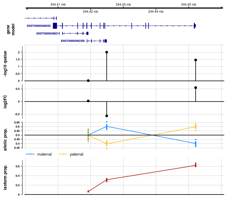
We can also customize the display of the alleles in the
plotInfReps() plots, by adding a new factor, while
carefully noting the existing and new allele labels, to make sure the
annotation is correct:
y$allele_new <- y$allele
# note a2 is non-effect, a1 is effect:
levels(y$allele)
## [1] "a2" "a1"
# replace a2 then a1:
levels(y$allele_new) <- c("maternal","paternal")
plotInfReps(y, idx=1, x="allele_new",
            legend=TRUE, legendPos="bottom")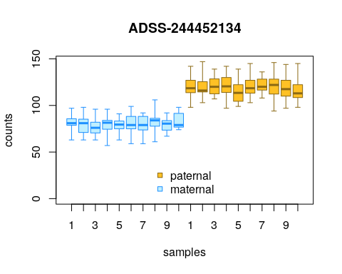
Differential allelic imbalance
Above, we tested for global AI, where the allelic fold change is
consistent across all samples. We can also test for differential or
dynamic AI, by adding specification of a cov (covariate)
which can be either a two-group factor, or a continuous variable. Here
we demonstrate differential AI, when cov is a two-group
factor, in this case called "condition".
set.seed(1)
y <- makeSimSwishData(diffAI=TRUE, n=12)
colData(y)
## DataFrame with 24 rows and 3 columns
## allele sample condition
## <factor> <factor> <factor>
## s1-a2 a2 sample1 A
## s2-a2 a2 sample2 A
## s3-a2 a2 sample3 A
## s4-a2 a2 sample4 A
## s5-a2 a2 sample5 A
## ... ... ... ...
## s8-a1 a1 sample8 B
## s9-a1 a1 sample9 B
## s10-a1 a1 sample10 B
## s11-a1 a1 sample11 B
## s12-a1 a1 sample12 B
table(y$condition, y$allele)##
## a2 a1
## A 6 6
## B 6 6In the following, we test for changes in allelic imbalance across
condition. This is implemented as an “interaction” test,
where we test if the fold change associated with allele,
for paired samples, differs across condition.
In this simulated data, the top two features exhibit differential AI with low uncertainty, so these emerge as highly significant, as expected.
mcols(y)[1:2,c("stat","qvalue")]## DataFrame with 2 rows and 2 columns
## stat qvalue
## <numeric> <numeric>
## gene-1 17.3 0.005
## gene-2 -17.5 0.005The non-AI features have roughly uniform p-values:
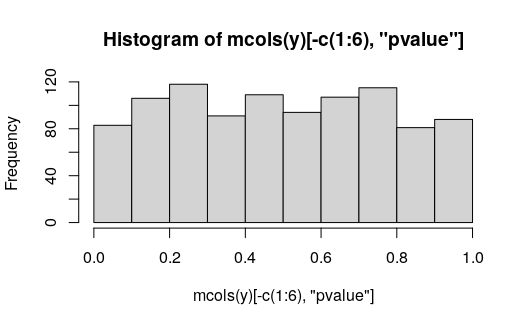
We can plot the allelic counts with uncertainty, grouped by the condition (black and grey lines at bottom).
plotInfReps(y, idx=1, x="allele", cov="condition",
            xaxis=FALSE, legend=TRUE, legendPos="bottomright")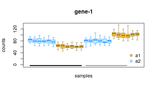
We can also visualize the data across multiple features, in terms of allelic ratios:
idx <- c(1:6)
row_dat <- data.frame(minusLogQ=-log10(mcols(y)$qvalue[idx]),
                      row.names=rownames(y)[idx])
col_dat <- data.frame(condition=y$condition[1:12],
                      row.names=paste0("s",1:12))
plotAllelicHeatmap(y, idx=idx,
                   annotation_row=row_dat,
                   annotation_col=col_dat,
                   cluster_rows=FALSE)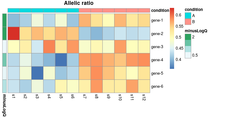
Dynamic allelic imbalance
Now we demonstrate dynamic AI testing when cov
(covariate) is a continuous variable. In this case, the user should
specify a correlation test, either cor="pearson" or
"spearman", which is the underlying test statistic used by
Swish (it will then be averaged over bootstraps and a permutation null
is generated to assess FDR). We have found that Pearson correlations
work well in our testing, but the Spearman correlation offers additional
robustness against outlying values in cov.
set.seed(1)
y <- makeSimSwishData(dynamicAI=TRUE)
colData(y)
## DataFrame with 20 rows and 3 columns
## allele sample time
## <factor> <factor> <numeric>
## s1-a2 a2 sample1 0.00
## s2-a2 a2 sample2 0.11
## s3-a2 a2 sample3 0.22
## s4-a2 a2 sample4 0.33
## s5-a2 a2 sample5 0.44
## ... ... ... ...
## s6-a1 a1 sample6 0.56
## s7-a1 a1 sample7 0.67
## s8-a1 a1 sample8 0.78
## s9-a1 a1 sample9 0.89
## s10-a1 a1 sample10 1.00A hidden code chunk adds ranges to our simulation data.
<hidden code chunk>In the following, we test for changes in allelic imbalance within
sample that correlate with a covariate time.
Note the first two features have small q-values and opposite test
statistic; here the test statistic is the average Pearson correlation of
the allelic log fold change with the time variable,
averaging over bootstrap replicates.
mcols(y)[1:2,c("stat","qvalue")]## DataFrame with 2 rows and 2 columns
## stat qvalue
## <numeric> <numeric>
## ADSS-244452134 0.870969 0.005
## ADSS-244419273 -0.861573 0.005For plotting inferential replicates over a continuous variable, we must first compute summary statistics of inferential mean and variance:
y <- computeInfRV(y)Now we can examine the allelic counts across the time
variable:
par(mfrow=c(2,1), mar=c(2.5,4,2,2))
plotInfReps(y, idx=1, x="time", cov="allele", shiftX=.01, xaxis=FALSE, xlab="", main="")
par(mar=c(4.5,4,0,2))
plotInfReps(y, idx=2, x="time", cov="allele", shiftX=.01, main="")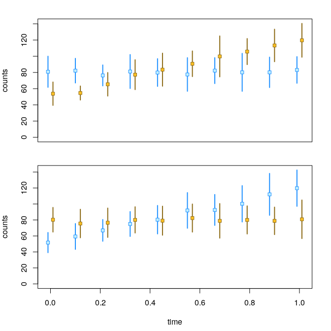
With a little more code, we can add a lowess line for
each series:
plotInfReps(y, idx=1, x="time", cov="allele", shiftX=.01)
dat <- data.frame(
  time = y$time[1:10],
  a2 = assay(y, "mean")[1,y$allele=="a2"],
  a1 = assay(y, "mean")[1,y$allele=="a1"])
lines(lowess(dat[,c(1,2)]), col="dodgerblue")
lines(lowess(dat[,c(1,3)]), col="goldenrod4")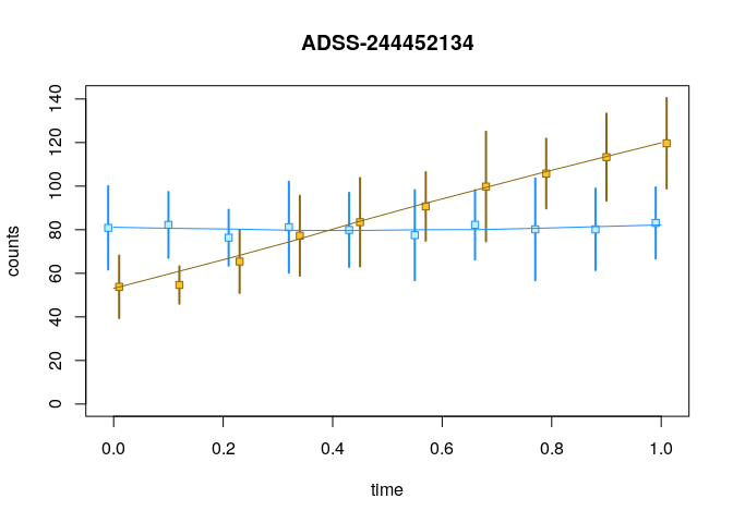
Visualizing the allelic proportion in a heatmap helps to see
relationships with the time variable, while also showing
data from multiple features at once:
idx <- c(1:4)
row_dat <- data.frame(minusLogQ=-log10(mcols(y)$qvalue[idx]),
                      row.names=rownames(y)[idx])
col_dat <- data.frame(time=y$time[1:10],
                      row.names=paste0("s",1:10))
plotAllelicHeatmap(y, idx=idx,
                   annotation_row=row_dat,
                   annotation_col=col_dat)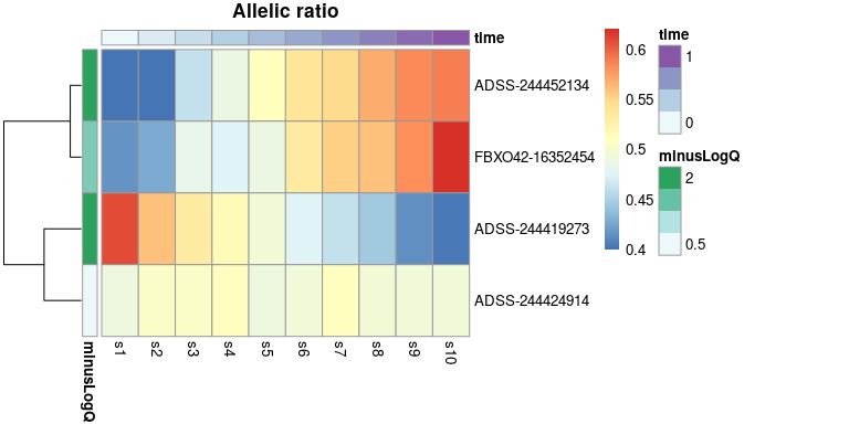
Plotting results in genomic context
Previously, in the global AI section, we demonstrated how to plot
TSS-level results in a genomic context using
plotAllelicGene(). Here we demonstrate how to repeat such a
plot for differential or dynamic AI analysis. There is an extra step for
dynamic analysis (binning the continuous covariate into groups) but
otherwise the code would be similar.
We begin by binning the time covariate into a few
groups, so that we can diagram the allelic and isoform proportions in
the genomic context, but facetting across time.
We create the binned covariate using cut, and rename the
labels for nicer labels in our plot. For differential AI, this step
would be skipped (as there already exists a two-group covariate for
grouping samples).
y$time_bins <- cut(y$time,breaks=c(0,.25,.75,1),
                   include.lowest=TRUE, labels=FALSE)
y$time_bins <- paste0("time-",y$time_bins)
table(y$time_bins[ y$allele == "a2" ])
##
## time-1 time-2 time-3
## 3 4 3We can then make our facetted allelic proportion plot:
gene <- rowRanges(y)$gene_id[1]
plotAllelicGene(y, gene, edb, cov="time_bins",
                qvalue=FALSE, log2FC=FALSE)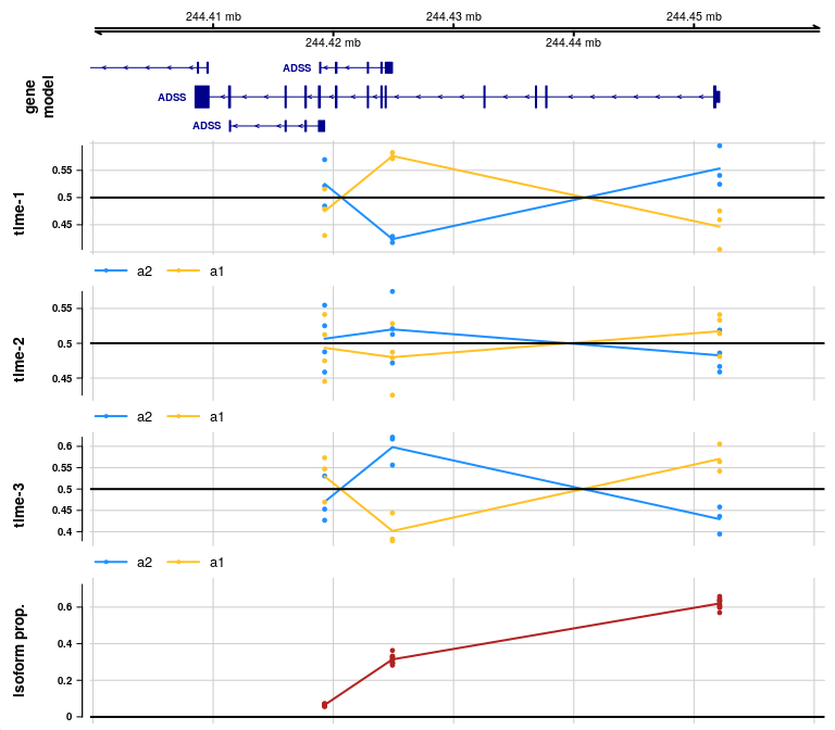
If we also want to visualize how isoform proportions may be changing,
we can add covFacetIsoform=TRUE, which additionally facets
the isoform proportion plot by the covariate:
plotAllelicGene(y, gene, edb, cov="time_bins",
                covFacetIsoform=TRUE,
                qvalue=FALSE, log2FC=FALSE)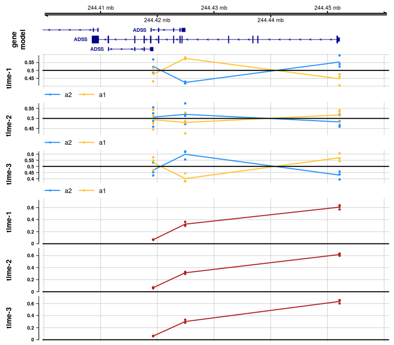
More complex designs
The SEESAW suite currently supports testing AI globally (across all samples), testing for differential AI (across two groups), or testing for dynamic AI (whether the allelic ratio changes over a continuous covariate such as time).
However, additional designs can also be used within the nonparametric
testing framework of Swish (and originally SAMseq).
The general idea of the testing framework is to compute a test
statistic, average that over inferential replicates, and then permute
the samples in order to generate a null distribution of the
bootstrap-averaged test statistic. The qvalue method and
package is then used to return the final inference. Here we explore
testing outside of swish function, by following these
steps. We will test for differential correlation of allelic ratios
across two groups.
First, we simulate a dataset with two groups, and insert differential correlation for one feature:
set.seed(1)
y1 <- makeSimSwishData(dynamicAI=TRUE)
y2 <- makeSimSwishData(dynamicAI=TRUE)
y2$sample <- factor(rep(paste0("sample",11:20),2))
y <- cbind(y1, y2)
y$group <- factor(rep(c("A","B"),each=20))
table(y$time, y$group) # 2 allelic counts per cell
##
## A B
## 0 2 2
## 0.11 2 2
## 0.22 2 2
## 0.33 2 2
## 0.44 2 2
## 0.56 2 2
## 0.67 2 2
## 0.78 2 2
## 0.89 2 2
## 1 2 2We change the direction of AI trend for the first feature:
reps <- grep("infRep", assayNames(y), value=TRUE)
for (k in reps) {
  assay(y,k)[1,21:40] <- assay(y,k)[1,c(31:40,21:30)]
}
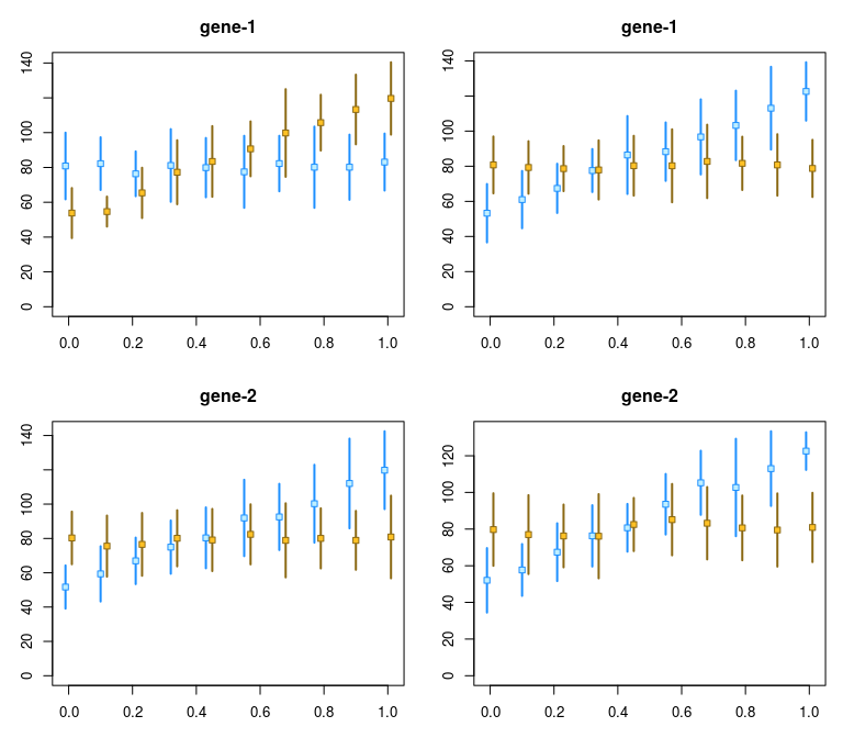
To visualize the differential correlation of AI with time for the first and second feature (left side, group A; right side, group B, features by row):
y <- computeInfRV(y)
par(mfrow=c(2,2),mar=c(3,3,3,1))
for (i in 1:2) {
  plotInfReps(y[,y$group=="A"], idx=i, x="time", cov="allele", shiftX=.01)
  plotInfReps(y[,y$group=="B"], idx=i, x="time", cov="allele", shiftX=.01)
}
We define a number of variables that will be used to compute test statistics:
pc <- 5 # a pseudocount
idx1 <- which(y$allele == "a1")
idx2 <- which(y$allele == "a2")
# the sample must be aligned
all.equal(y$sample[idx1], y$sample[idx2])
## [1] TRUE
cov <- y$time[idx1]
group <- y$group[idx1]
# interaction of group and covariate (time)
design <- model.matrix(~group + cov + group:cov)
For efficiency, we precompute the allelic LFC array (features x samples x infReps):
reps <- grep("infRep", assayNames(y), value=TRUE)
nreps <- length(reps)
infReps <- assays(y)[reps]
infRepsArray <- abind::abind(as.list(infReps), along=3)
lfcArray <- log2(infRepsArray[,idx1,] + pc) -
            log2(infRepsArray[,idx2,] + pc)
For the statistic, we extract the coefficient for the interaction of
group and the time covariate, using limma::lmFit applied to
a matrix of log2 fold changes. We then compute basic t-statistics from
this table of linear model coefficients. It is useful to define a
function to repeat this operation (over inferential replicates and
permutations).
computeStat <- function(k, design, name) {
  fit <- limma::lmFit(lfcArray[,,k], design)
  tstats <- fit$coef/fit$stdev.unscaled/fit$sigma
  tstats[,name]
}
We then use the SAMseq/Swish strategy to average over the inferential replicates, for the observed data:
Finally, we repeat, while permuting the group labels for the samples 100 times:
n <- nrow(design)
nperms <- 100
nulls <- matrix(nrow=nrow(y), ncol=nperms)
set.seed(1)
for (p in seq_len(nperms)) {
  # permute group labels
  pgroup <- group[sample(n)]
  pdesign <- model.matrix(~pgroup + cov + pgroup:cov)
  nulls[,p] <- rowMeans(sapply(1:nreps, \(k) computeStat(k, pdesign, "pgroupB:cov")))
}
The rest of the process is providing the observed statistic and the
null statistics to the qvalue function:
pvalue <- qvalue::empPvals(abs(stat), abs(nulls))
q_res <- qvalue::qvalue(pvalue)
locfdr <- q_res$lfdr
qvalue <- q_res$qvalues
res <- data.frame(stat, pvalue, locfdr, qvalue)
We can see the first feature is retained with a low q-value while the others show a relatively flat histogram of p-values.
head(res)## stat pvalue locfdr qvalue
## gene-1 -6.89602993 0.00001 0.0388765 0.0100000
## gene-2 -0.08979129 0.70415 1.0000000 0.9913997
## gene-3 -0.16623033 0.48227 1.0000000 0.9772813
## gene-4 0.04186206 0.85828 1.0000000 0.9980000
## gene-5 -0.13609701 0.56461 1.0000000 0.9772813
## gene-6 0.15545421 0.51181 1.0000000 0.9772813
hist(res$pvalue[-1])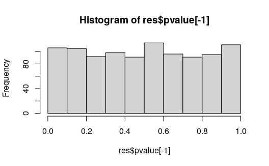
This general process for extracting arbitrary statistics on the allelic log fold change and making use of permutation for generating q-values can be applied to various designs.
Further questions
For further questions about the SEESAW steps, please post to one of these locations:
- Bioconductor support site https://support.bioconductor.org and use the tag
fishpondorswish - GitHub Issue https://github.com/mikelove/fishpond
Session info
## R Under development (unstable) (2024-12-25 r87466)
## Platform: x86_64-pc-linux-gnu
## Running under: Ubuntu 24.04.1 LTS
##
## Matrix products: default
## BLAS:   /usr/lib/x86_64-linux-gnu/openblas-pthread/libblas.so.3
## LAPACK: /usr/lib/x86_64-linux-gnu/openblas-pthread/libopenblasp-r0.3.26.so;  LAPACK version 3.12.0
##
## locale:
##  [1] LC_CTYPE=en_US.UTF-8       LC_NUMERIC=C
##  [3] LC_TIME=en_US.UTF-8        LC_COLLATE=en_US.UTF-8
##  [5] LC_MONETARY=en_US.UTF-8    LC_MESSAGES=en_US.UTF-8
##  [7] LC_PAPER=en_US.UTF-8       LC_NAME=C
##  [9] LC_ADDRESS=C               LC_TELEPHONE=C
## [11] LC_MEASUREMENT=en_US.UTF-8 LC_IDENTIFICATION=C
##
## time zone: UTC
## tzcode source: system (glibc)
##
## attached base packages:
## [1] stats4    stats     graphics  grDevices utils     datasets  methods
## [8] base
##
## other attached packages:
##  [1] SummarizedExperiment_1.37.0 MatrixGenerics_1.19.0
##  [3] matrixStats_1.4.1           fishpond_2.7.5
##  [5] EnsDb.Hsapiens.v86_2.99.0   ensembldb_2.31.0
##  [7] AnnotationFilter_1.31.0     GenomicFeatures_1.59.1
##  [9] AnnotationDbi_1.69.0        Biobase_2.67.0
## [11] GenomicRanges_1.59.1        GenomeInfoDb_1.43.2
## [13] IRanges_2.41.2              S4Vectors_0.45.2
## [15] BiocGenerics_0.53.3         generics_0.1.3
##
## loaded via a namespace (and not attached):
##   [1] RColorBrewer_1.1-3          rstudioapi_0.17.1
##   [3] jsonlite_1.8.9              magrittr_2.0.3
##   [5] farver_2.1.2                rmarkdown_2.29
##   [7] fs_1.6.5                    BiocIO_1.17.1
##   [9] zlibbioc_1.53.0             ragg_1.3.3
##  [11] vctrs_0.6.5                 memoise_2.0.1
##  [13] Rsamtools_2.23.1            RCurl_1.98-1.16
##  [15] base64enc_0.1-3             htmltools_0.5.8.1
##  [17] S4Arrays_1.7.1              progress_1.2.3
##  [19] curl_6.0.1                  SparseArray_1.7.2
##  [21] Formula_1.2-5               sass_0.4.9
##  [23] bslib_0.8.0                 htmlwidgets_1.6.4
##  [25] desc_1.4.3                  plyr_1.8.9
##  [27] Gviz_1.51.0                 httr2_1.0.7
##  [29] cachem_1.1.0                GenomicAlignments_1.43.0
##  [31] lifecycle_1.0.4             pkgconfig_2.0.3
##  [33] Matrix_1.7-1                R6_2.5.1
##  [35] fastmap_1.2.0               GenomeInfoDbData_1.2.13
##  [37] digest_0.6.37               colorspace_2.1-1
##  [39] textshaping_0.4.1           Hmisc_5.2-1
##  [41] RSQLite_2.3.9               filelock_1.0.3
##  [43] httr_1.4.7                  abind_1.4-8
##  [45] compiler_4.5.0              bit64_4.5.2
##  [47] htmlTable_2.4.3             backports_1.5.0
##  [49] BiocParallel_1.41.0         DBI_1.2.3
##  [51] biomaRt_2.63.0              rappdirs_0.3.3
##  [53] DelayedArray_0.33.3         rjson_0.2.23
##  [55] gtools_3.9.5                tools_4.5.0
##  [57] foreign_0.8-87              nnet_7.3-20
##  [59] glue_1.8.0                  restfulr_0.0.15
##  [61] grid_4.5.0                  checkmate_2.3.2
##  [63] cluster_2.1.8               reshape2_1.4.4
##  [65] gtable_0.3.6                BSgenome_1.75.0
##  [67] data.table_1.16.4           hms_1.1.3
##  [69] xml2_1.3.6                  XVector_0.47.1
##  [71] pillar_1.10.0               stringr_1.5.1
##  [73] limma_3.63.2                splines_4.5.0
##  [75] dplyr_1.1.4                 BiocFileCache_2.15.0
##  [77] lattice_0.22-6              deldir_2.0-4
##  [79] rtracklayer_1.67.0          bit_4.5.0.1
##  [81] biovizBase_1.55.0           tidyselect_1.2.1
##  [83] SingleCellExperiment_1.29.1 Biostrings_2.75.3
##  [85] knitr_1.49                  gridExtra_2.3
##  [87] ProtGenerics_1.39.1         xfun_0.49
##  [89] statmod_1.5.0               pheatmap_1.0.12
##  [91] stringi_1.8.4               UCSC.utils_1.3.0
##  [93] lazyeval_0.2.2              yaml_2.3.10
##  [95] evaluate_1.0.1              codetools_0.2-20
##  [97] interp_1.1-6                tibble_3.2.1
##  [99] qvalue_2.39.0               cli_3.6.3
## [101] rpart_4.1.23                systemfonts_1.1.0
## [103] munsell_0.5.1               jquerylib_0.1.4
## [105] dichromat_2.0-0.1           Rcpp_1.0.13-1
## [107] svMisc_1.4.3                dbplyr_2.5.0
## [109] png_0.1-8                   XML_3.99-0.18
## [111] parallel_4.5.0              pkgdown_2.1.1
## [113] ggplot2_3.5.1               blob_1.2.4
## [115] prettyunits_1.2.0           jpeg_0.1-10
## [117] latticeExtra_0.6-30         bitops_1.0-9
## [119] VariantAnnotation_1.53.0    scales_1.3.0
## [121] crayon_1.5.3                rlang_1.1.4
## [123] KEGGREST_1.47.0