tximeta: transcript quantification import with automatic metadata
Michael I. Love, Charlotte Soneson, Peter F. Hickey, Rob Patro
07/08/2026
Source:vignettes/tximeta.Rmd
tximeta.RmdAbstract
tximeta performs numerous annotation and metadata gathering tasks on behalf of users during the import of transcript counts and abundance from quantification tools such as salmon. Data are imported as SummarizedExperiment objects with associated GenomicRanges metadata. Correct metadata is added automatically via reference sequence digests, facilitating genomic analyses and assisting in computational reproducibility. Addition functionality is now offered for quantification with mixed reference transcripts, e.g. GENCODE plus novel transcripts.
If viewing vignette on Bioconductor, see here for a nicely rendered version.
Introduction
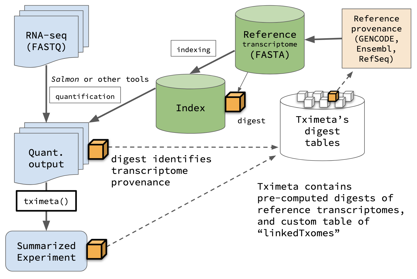
The tximeta package (Love et al. 2020) extends the tximport package (Soneson et al. 2015) for import of transcript-level quantification data into R/Bioconductor. It automatically adds annotation metadata when the RNA-seq data has been quantified with salmon (Patro et al. 2017) or related tools. To our knowledge, tximeta is the only package for RNA-seq data import that can automatically identify and attach transcriptome metadata based on the unique sequence collection of the reference transcripts. For more details on these packages – including the motivation for tximeta and description of similar work – consult the References below.
Note: For details of using tximeta
functions with oarfish, in particular
with separate --annotated and --novel
reference transcripts, refer to this section below.
Note: tximeta() requires that the
entire output of the quantificaation tool is present in
the output directories and unmodified in order to identify the
provenance of the reference transcripts. In general, it’s a good idea to
not modify or re-arrange the output directory of bioinformatic software
as other downstream software often rely on and assume a consistent
directory structure. For sharing multiple samples, one can use, for
example, tar -czf to bundle up a set of salmon
output directories. For tips on using tximeta() with other
quantifiers see the other quantifiers
section below.
Preparing tximeta input
The first step using tximeta() is to read in the sample
table, which will become the column data, colData,
of the final object, a SummarizedExperiment. The sample table
should contain all the information we need to identify the
salmon quantification directories.
Here we will use a salmon quantification file in the
tximportData package to demonstrate the usage of
tximeta. We do not have a sample table, so we construct one
in R. It is recommended to keep a sample table as a CSV or TSV file
while working on an RNA-seq project with multiple samples.
dir <- system.file("extdata/salmon_dm", package="tximportData")
files <- file.path(dir, "SRR1197474", "quant.sf")
file.exists(files)
## [1] TRUE
coldata <- data.frame(files, names="SRR1197474", condition="A", stringsAsFactors=FALSE)
coldata
## files
## 1 /__w/_temp/Library/tximportData/extdata/salmon_dm/SRR1197474/quant.sf
## names condition
## 1 SRR1197474 Atximeta() expects at least two columns in
coldata:
-
files- a pointer to thequant.sffiles -
names- the unique names that should be used to identify samples
Other columns will be propagated to colData of the
SummarizedExperiment output.
Running tximeta
Normally, we would just run tximeta like so:
However, to avoid downloading remote GTF files during this vignette,
we will point to a GTF file saved locally (in the tximportData
package). We link the transcriptome of the salmon index to its
locally saved GTF. The standard recommended usage of
tximeta(),
in particular for quantification with reference transcripts with a pre-computed digest, would be the code
chunk above. If one were adding another set of reference transcripts,
one would normally specify a remote GTF source, not a local one.
This following code is therefore not recommended for a typical
workflow, but is particular to the vignette code.
indexDir <- file.path(dir, "Dm.BDGP6.22.98_salmon-0.14.1")
fastaFTP <- c("ftp://ftp.ensembl.org/pub/release-98/fasta/drosophila_melanogaster/cdna/Drosophila_melanogaster.BDGP6.22.cdna.all.fa.gz",
              "ftp://ftp.ensembl.org/pub/release-98/fasta/drosophila_melanogaster/ncrna/Drosophila_melanogaster.BDGP6.22.ncrna.fa.gz")
gtfPath <- file.path(dir,"Drosophila_melanogaster.BDGP6.22.98.gtf.gz")
suppressPackageStartupMessages(library(tximeta))
makeLinkedTxome(indexDir=indexDir,
                source="LocalEnsembl",
                organism="Drosophila melanogaster",
                release="98",
                genome="BDGP6.22",
                fasta=fastaFTP,
                gtf=gtfPath,
                write=FALSE)
## reading digest from indexDir: .../Dm.BDGP6.22.98_salmon-0.14.1## NOTE: this digest matches one in the pre-computed digest table## saving linkedTxome in bfc (first time)
se <- tximeta(coldata)## importing salmon quantification files## reading in files with read.delim (install 'readr' package for speed up)## 1
## found matching linkedTxome:
## [ LocalEnsembl - Drosophila melanogaster - release 98 ]
## building TxDb with 'txdbmaker' package
## Import genomic features from the file as a GRanges object ... OK
## Prepare the 'metadata' data frame ... OK
## Make the TxDb object ...## Warning in .makeTxDb_normarg_chrominfo(chrominfo): genome version information
## is not available for this TxDb object## OK
## generating transcript ranges## Warning in checkAssays2Txps(assays, txps):
##
## Warning: the annotation is missing some transcripts that were quantified.
## 5 out of 33706 txps were missing from GTF/GFF but were in the indexed FASTA
## (e.g. this can occur with transcripts located on haplotype chromosomes).
## In order to build a ranged SummarizedExperiment, these txps were removed.
## To keep these txps, and to skip adding ranges, use skipMeta=TRUE
##
## Example missing txps: [FBtr0307759, FBtr0084079, FBtr0084080, ...]This warning, “Warning: the annotation is missing some
transcripts that were quantified.”, is common and occurs when
annotation sources provide transcripts in the FASTA file that aren’t
annotated in the GTF file. This is upstream of tximeta(),
but this package will notify you the number of transcripts for which
this is the case.
How does it work?
tximeta() recognized the computed digest of the
transcriptome that the files were quantified against, it accessed the
GTF file of the transcriptome source, found and attached the transcript
ranges, and added the appropriate transcriptome and genome metadata. A
digest is a small string of alphanumeric characters that
uniquely identifies the collection of sequences that were used for
quantification (it is the hash value from applying the hash function to
a particular collection of nucleotide sequences). We sometimes also call
this value a “checksum” (in the tximeta paper), and we sometimes call
the table of pre-computed digests or linked digests a “hash table”.
Note that a remote GTF is only downloaded once, and a local or remote
GTF is only parsed to build a TxDb or EnsDb once: if
tximeta() recognizes that it has seen this salmon
index before, it will use a cached version of the metadata and
transcript ranges.
Packages used for caching metadata
tximeta() makes use of Bioconductor packages for storing
transcript databases as TxDb or EnsDb objects, which
both are connected by default to sqlite backends. For
GENCODE and RefSeq GTF files, tximeta() uses the
txdbmaker package to parse the GTF and build a TxDb.
For Ensembl GTF files, tximeta() will first attempt to
obtain the correct EnsDb object using AnnotationHub.
The ensembldb package (Rainer et al.
2019) contains classes and methods for extracting relevant data
from Ensembl files. If the EnsDb has already been made
available on AnnotationHub, tximeta() will download the
database directly, which saves the user time parsing the GTF into a
database (to avoid this, set useHub=FALSE). If the relevant
EnsDb is not available on AnnotationHub, tximeta()
will build an EnsDb using ensembldb after downloading
the GTF file. Again, the download/construction of a transcript database
occurs only once, and upon subsequent usage of tximeta
functions, the cached version will be used.
Pre-computed digests
The following digests for human, mouse, and drosophila reference
transcripts are supported in this version of tximeta():
| source | organism | releases |
|---|---|---|
| GENCODE | Homo sapiens | 23-50 |
| GENCODE | Mus musculus | M6-M39 |
| Ensembl | Homo sapiens | 76-116 |
| Ensembl | Mus musculus | 76-116 |
| Ensembl | Drosophila melanogaster | 79-115 |
| RefSeq | Homo sapiens | p1-p13 |
| RefSeq | Mus musculus | p2-p6 |
For Ensembl transcriptomes, we support the combined protein coding (cDNA) and non-coding (ncRNA) sequences, as well as the protein coding alone (although the former approach combining coding and non-coding transcripts is recommended for more accurate quantification).
tximeta() also supports linked transcriptomes,
a mechanism to link quantification data to key metadata. This can be
used to resolve many potential situations where one of the above
pre-computed digests won’t be a match (due to modifying, re-ordering,
adding, or removing transcripts, which changes the value of the compute
digest). See the Linked
transcriptomes section below for a demonstration. (The
makeLinkedTxome function was used above to avoid downloading
the GTF during the vignette building process.)
For oarfish quantification (Zare
Jousheghani et al. 2025) using the --annotated and
--novel reference transcripts, use the functions described
below.
SummarizedExperiment output
The SummarizedExperiment object resulting from the data
import contains our coldata from before. Note that the
files column was removed during the import.
## DataFrame with 1 row and 2 columns
##                  names   condition
##            <character> <character>
## SRR1197474  SRR1197474           A
Here we show the three matrices that were imported.
assayNames(se)## [1] "counts" "abundance" "length"If there were inferential replicates (Gibbs samples or bootstrap
samples), these would be imported as additional assays named
"infRep1", "infRep2", …
tximeta() has imported the correct ranges for the
transcripts:
rowRanges(se)## GRanges object with 33701 ranges and 3 metadata columns:
## seqnames ranges strand | tx_id gene_id
## <Rle> <IRanges> <Rle> | <integer> <CharacterList>
## FBtr0070129 X 656673-657899 + | 28756 FBgn0025637
## FBtr0070126 X 656356-657899 + | 28752 FBgn0025637
## FBtr0070128 X 656673-657899 + | 28755 FBgn0025637
## FBtr0070124 X 656114-657899 + | 28750 FBgn0025637
## FBtr0070127 X 656356-657899 + | 28753 FBgn0025637
## ... ... ... ... . ... ...
## FBtr0114299 2R 21325218-21325323 + | 9300 FBgn0086023
## FBtr0113582 3R 5598638-5598777 - | 24474 FBgn0082989
## FBtr0091635 3L 1488906-1489045 + | 13780 FBgn0086670
## FBtr0113599 3L 261803-261953 - | 16973 FBgn0083014
## FBtr0113600 3L 831870-832008 - | 17070 FBgn0083057
## tx_name
## <character>
## FBtr0070129 FBtr0070129
## FBtr0070126 FBtr0070126
## FBtr0070128 FBtr0070128
## FBtr0070124 FBtr0070124
## FBtr0070127 FBtr0070127
## ... ...
## FBtr0114299 FBtr0114299
## FBtr0113582 FBtr0113582
## FBtr0091635 FBtr0091635
## FBtr0113599 FBtr0113599
## FBtr0113600 FBtr0113600
## -------
## seqinfo: 25 sequences from an unspecified genome; no seqlengthsWe have appropriate genome information, which prevents us from making bioinformatic mistakes:
seqinfo(se)## Seqinfo object with 25 sequences from an unspecified genome; no seqlengths:
## seqnames seqlengths isCircular genome
## 2L <NA> <NA> <NA>
## 2R <NA> <NA> <NA>
## 3L <NA> <NA> <NA>
## 3R <NA> <NA> <NA>
## 4 <NA> <NA> <NA>
## ... ... ... ...
## 211000022280481 <NA> <NA> <NA>
## 211000022280494 <NA> <NA> <NA>
## 211000022280703 <NA> <NA> <NA>
## mitochondrion_genome <NA> <NA> <NA>
## rDNA <NA> <NA> <NA>Retrieve the transcript database
The se object has associated metadata that allows
tximeta to link to locally stored cached databases and
other Bioconductor objects. In further sections, we will show examples
of functions that leverage these databases to add exon information,
summarize transcript-level data to the gene level, or add identifiers.
However, first we mention that the user can easily access the cached
database with the following helper function. In this case,
tximeta has an associated EnsDb object that we can
retrieve and use in our R session:
edb <- retrieveDb(se)## loading existing TxDb created: 2026-07-08 20:46:51
class(edb)## [1] "TxDb"
## attr(,"package")
## [1] "GenomicFeatures"The database returned by retrieveDb is either a
TxDb in the case of GENCODE or RefSeq GTF annotation file, or
an EnsDb in the case of an Ensembl GTF annotation file. For
further use of these two database objects, consult the
GenomicFeatures vignettes and the ensembldb vignettes,
respectively (both Bioconductor packages).
Add exons per transcript
Because the SummarizedExperiment maintains all the metadata of its creation, it also keeps a pointer to the necessary database for pulling out additional information, as demonstrated in the following sections.
If necessary, the tximeta package can pull down the remote
source to build a TxDb, but given that we’ve already built a TxDb once,
it simply loads the cached version. In order to remove the cached TxDb
and regenerate, one can remove the relevant entry from the
tximeta file cache that resides at the location given by
getTximetaBFC().
The se object created by tximeta, has the
start, end, and strand information for each transcript. Here, we swap
out the transcript GRanges for exons-by-transcript
GRangesList (it is a list of GRanges, where each
element of the list gives the exons for a particular transcript).
se.exons <- addExons(se)## loading existing TxDb created: 2026-07-08 20:46:51## generating exon ranges
rowRanges(se.exons)[[1]]## GRanges object with 2 ranges and 3 metadata columns:
## seqnames ranges strand | exon_id exon_name exon_rank
## <Rle> <IRanges> <Rle> | <integer> <character> <integer>
## [1] X 656673-656740 + | 72949 FBtr0070129-E1 1
## [2] X 657099-657899 + | 72952 FBtr0070129-E2 2
## -------
## seqinfo: 25 sequences from an unspecified genome; no seqlengthsAs with the transcript ranges, the exon ranges will be generated once
and cached locally. As it takes a non-negligible amount of time to
generate the exon-by-transcript GRangesList, this local caching
offers substantial time savings for repeated usage of
addExons with the same transcriptome.
We have implemented addExons to work only on the
transcript-level SummarizedExperiment object. We provide some
motivation for this choice in ?addExons. Briefly, if it is
desired to know the exons associated with a particular gene, we feel
that it makes more sense to pull out the relevant set of
exons-by-transcript for the transcripts for this gene, rather than
losing the hierarchical structure (exons to transcripts to genes) that
would occur with a GRangesList of exons grouped per gene.
Easy summarization to gene-level
Likewise, the tximeta package can make use of the cached
TxDb database for the purpose of summarizing transcript-level
quantifications and bias corrections to the gene-level. After
summarization, the rowRanges reflect the start and end
position of the gene, which in Bioconductor are defined by the leftmost
and rightmost genomic coordinates of all the transcripts. As with the
transcript and exons, the gene ranges are cached locally for repeated
usage. The transcript IDs are stored as a CharacterList column
tx_ids.
Note: you can also use summarizeToGene
on an object created with skipMeta=TRUE which therefore
does not have ranges or an associated TxDb by setting
skipRanges=TRUE and providing your own tx2gene
table which is passed to tximport.
gse <- summarizeToGene(se)## loading existing TxDb created: 2026-07-08 20:46:51## obtaining transcript-to-gene mapping from database## generating gene ranges## assignRanges='range': gene ranges assigned by total range of isoforms
## see details at: ?summarizeToGene,SummarizedExperiment-method## summarizing abundance## summarizing counts## summarizing length
rowRanges(gse)## GRanges object with 17208 ranges and 2 metadata columns:
## seqnames ranges strand | gene_id
## <Rle> <IRanges> <Rle> | <character>
## FBgn0000003 3R 6822498-6822796 + | FBgn0000003
## FBgn0000008 2R 22136968-22172834 + | FBgn0000008
## FBgn0000014 3R 16807214-16830049 - | FBgn0000014
## FBgn0000015 3R 16927212-16972236 - | FBgn0000015
## FBgn0000017 3L 16615866-16647882 - | FBgn0000017
## ... ... ... ... . ...
## FBgn0286199 3R 24279572-24281576 + | FBgn0286199
## FBgn0286203 2R 5413744-5456095 + | FBgn0286203
## FBgn0286204 3R 8950246-8963037 - | FBgn0286204
## FBgn0286213 3L 13023352-13024762 + | FBgn0286213
## FBgn0286222 X 6678424-6681845 + | FBgn0286222
## tx_ids
## <CharacterList>
## FBgn0000003 FBtr0081624
## FBgn0000008 FBtr0071763,FBtr0100521,FBtr0342981,...
## FBgn0000014 FBtr0306337,FBtr0083388,FBtr0083387,...
## FBgn0000015 FBtr0415463,FBtr0415464,FBtr0083385,...
## FBgn0000017 FBtr0112790,FBtr0345369,FBtr0075357,...
## ... ...
## FBgn0286199 FBtr0084600
## FBgn0286203 FBtr0299918,FBtr0299920,FBtr0299921,...
## FBgn0286204 FBtr0082014,FBtr0334329
## FBgn0286213 FBtr0075878
## FBgn0286222 FBtr0070953,FBtr0070954
## -------
## seqinfo: 25 sequences from an unspecified genome; no seqlengthsAssign ranges by abundance
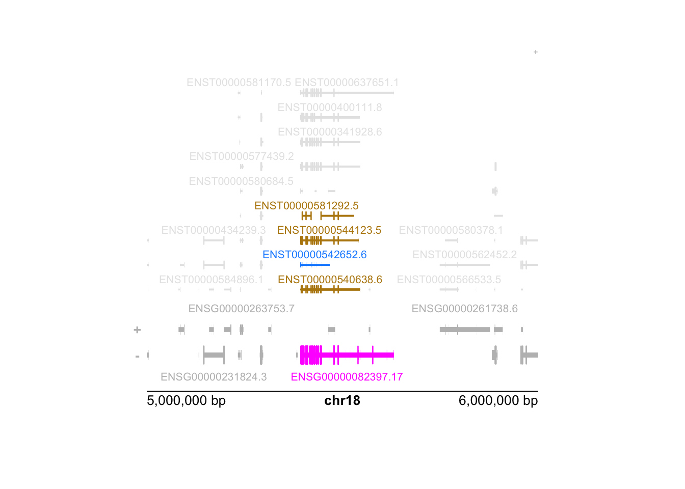
We also offer a new type of range assignment, based on the most
abundant isoform rather than the leftmost to rightmost coordinate. See
the assignRanges argument of ?summarizeToGene.
Using the most abundant isoform arguably will reflect more accurate
genomic distances than the default option.
# unevaluated code chunk
gse <- summarizeToGene(se, assignRanges="abundant")
For more explanation about why this may be a better choice, see the following tutorial chapter:
https://tidyomics.github.io/tidy-ranges-tutorial/gene-ranges-in-tximeta.html
In the below diagram, the pink feature is the set of all exons belonging to any isoform of the gene, such that the TSS is on the right side of this minus strand feature. However, the blue feature is the most abundant isoform (the brown features are the next most abundant isoforms). The pink feature is therefore not a good representation for the locus.
Add different identifiers
We would like to add support to easily map transcript or gene identifiers from one annotation to another. This is just a prototype function, but we show how we can easily add alternate IDs given that we know the organism and the source of the transcriptome. (This function currently only works for GENCODE and Ensembl gene or transcript IDs but could be extended to work for arbitrary sources.)
library(org.Dm.eg.db)##
gse <- addIds(gse, "REFSEQ", gene=TRUE)## mapping to new IDs using org.Dm.eg.db
## if all matching IDs are desired, and '1:many mappings' are reported,
## set multiVals='list' to obtain all the matching IDs## 'select()' returned 1:many mapping between keys and columns
mcols(gse)## DataFrame with 17208 rows and 3 columns
## gene_id tx_ids REFSEQ
## <character> <CharacterList> <character>
## FBgn0000003 FBgn0000003 FBtr0081624 NR_001992
## FBgn0000008 FBgn0000008 FBtr0071763,FBtr0100521,FBtr0342981,... NM_001014543
## FBgn0000014 FBgn0000014 FBtr0306337,FBtr0083388,FBtr0083387,... NM_001170161
## FBgn0000015 FBgn0000015 FBtr0415463,FBtr0415464,FBtr0083385,... NM_001275719
## FBgn0000017 FBgn0000017 FBtr0112790,FBtr0345369,FBtr0075357,... NM_001104153
## ... ... ... ...
## FBgn0286199 FBgn0286199 FBtr0084600 NM_142982
## FBgn0286203 FBgn0286203 FBtr0299918,FBtr0299920,FBtr0299921,... NM_001144134
## FBgn0286204 FBgn0286204 FBtr0082014,FBtr0334329 NM_001275464
## FBgn0286213 FBgn0286213 FBtr0075878 NM_168534
## FBgn0286222 FBgn0286222 FBtr0070953,FBtr0070954 NM_132111Differential gene expression analysis
The following code chunk demonstrates how to build a DESeqDataSet and begin a differential expression analysis with genewise counts.
suppressPackageStartupMessages(library(DESeq2))
# here there is a single sample so we use ~1.
# expect a warning that there is only a single sample...
suppressWarnings({dds <- DESeqDataSet(gse, ~1)})
# ... see DESeq2 vignette
The following code demonstrates how build a DGEList object for use with edgeR or limma-voom.
suppressPackageStartupMessages(library(edgeR))
y <- DGEListFromTximeta(gse)
# ... see edgeR or limma User's Guide for further steps
Above we generated counts-from-abundance when calling
summarizeToGene. The counts-from-abundance status is then
stored in the metadata:
metadata(gse)$countsFromAbundance ## [1] "no"Differential transcript expression and usage analysis
The Swish method in the fishpond package directly
works with the SummarizedExperiment output from
tximeta, and can perform differential analysis on transcript
expression taking into account inferential replicates, e.g. bootstrap or
Gibbs samples, which are imported and arranged by tximeta
if these were generated during quantification.
library(fishpond)
y <- se
y <- scaleInfReps(y)
y <- labelKeep(y)
y <- swish(y, x="condition")
# ... see Swish vignette in fishpond package
The edgeR::DGEListFromTximeta function uses the
inferential replicates found in se or gse to
estimate the overdispersion for each transcript or gene arising from the
fact that reads have to be assigned probabilistically to transcripts by
the quantification software (salmon in this case). The
DGEListFromTximeta function is available in edgeR
as of version 4.10.0 (Bioconductor release 3.23, Spring 2026).
Differential analyses of transcript expression or usage can be conducted
in edgeR or limma using “divided counts”, whereby the
overdispersion is divided out of the counts (Baldoni et al. 2024, 2025). The following code
produces a DGEList object suitable for transcript-level
analysis in edgeR or limma.
y <- DGEListFromTximeta(se, divide = TRUE)
# ... see edgeR or limma User's Guide for further steps
Additional metadata slots
The following information is attached to the
SummarizedExperiment by tximeta:
## [1] "tximetaInfo"         "quantInfo"           "countsFromAbundance"
## [4] "level" "txomeInfo" "txdbInfo"## List of 31
## $ salmon_version : chr "0.14.1"
## $ samp_type : chr "none"
## $ opt_type : chr "vb"
## $ quant_errors :List of 1
## ..$ : list()
## $ num_libraries : int 1
## $ library_types : chr "ISR"
## $ frag_dist_length : int 1001
## $ seq_bias_correct : logi FALSE
## $ gc_bias_correct : logi TRUE
## $ num_bias_bins : int 4096
## $ mapping_type : chr "mapping"
## $ num_valid_targets : int 33706
## $ num_decoy_targets : int 0
## $ num_eq_classes : int 70718
## $ serialized_eq_classes : logi FALSE
## $ length_classes : int [1:5, 1] 867 1533 2379 3854 71382
## $ index_seq_hash : chr "7ba5e9597796ea86cf11ccf6635ca88fbc37c2848d38083c23986aa2c6a21eae"
## $ index_name_hash : chr "b6426061057bba9b7afb4dc76fa68238414cf35b4190c95ca6fc44280d4ca87c"
## $ index_seq_hash512 : chr "05f111abcda1efd2e489ace6324128cdaaa311712a28ed716d957fdfd8706ec41ca9177ebf12f54e99c2a89582d06f31c5e09dc1dce2d13"| __truncated__
## $ index_name_hash512 : chr "ccdf58f23e48c8c53cd122b5f5990b5adce9fec87ddf8bd88153afbe93296d87b818fba89d12dbc20c882f7d98353840394c5040fea7432"| __truncated__
## $ num_bootstraps : int 0
## $ num_processed : int 42422337
## $ num_mapped : int 34098209
## $ num_decoy_fragments : int 0
## $ num_dovetail_fragments : int 2048810
## $ num_fragments_filtered_vm : int 989383
## $ num_alignments_below_threshold_for_mapped_fragments_vm: int 267540
## $ percent_mapped : num 80.4
## $ call : chr "quant"
## $ start_time : chr "Sat Oct 12 13:55:01 2019"
## $ end_time : chr "Sat Oct 12 14:08:11 2019"## List of 10
## $ index : chr "Dm.BDGP6.22.98_salmon-0.14.1"
## $ source : chr "LocalEnsembl"
## $ organism : chr "Drosophila melanogaster"
## $ release : chr "98"
## $ genome : chr "BDGP6.22"
## $ fasta :List of 1
## ..$ : chr [1:2] "ftp://ftp.ensembl.org/pub/release-98/fasta/drosophila_melanogaster/cdna/Drosophila_melanogaster.BDGP6.22.cdna.all.fa.gz" "ftp://ftp.ensembl.org/pub/release-98/fasta/drosophila_melanogaster/ncrna/Drosophila_melanogaster.BDGP6.22.ncrna.fa.gz"
## $ gtf : chr "/__w/_temp/Library/tximportData/extdata/salmon_dm/Drosophila_melanogaster.BDGP6.22.98.gtf.gz"
## $ sha256 : chr "7ba5e9597796ea86cf11ccf6635ca88fbc37c2848d38083c23986aa2c6a21eae"
## $ linkedTxome : Named logi TRUE
## ..- attr(*, "names")= chr "txome"
## $ linkedTxpData: Named logi FALSE
## ..- attr(*, "names")= chr "txome"## List of 3
## $ version :Classes 'package_version', 'numeric_version' hidden list of 1
## ..$ : int [1:3] 1 31 6
## $ type : chr "salmon"
## $ importTime: POSIXct[1:1], format: "2026-07-08 20:46:43"## Named chr [1:12] "TxDb" "GenomicFeatures" ...
## - attr(*, "names")= chr [1:12] "Db type" "Supporting package" "Data source" "Organism" ...Mixed reference transcripts
The oarfish (Zare Jousheghani et al. 2025) quantification tool and salmon allow specifying distinct annotated reference transcripts (e.g. GENCODE, Ensembl) and novel reference transcripts (e.g. de novo assemblies) which are combined together as the index for alignment and quantification. tximeta can now automatically recognize the provenance of reference transcripts even when sets from different sources are combined.
For example, oarfish code for indexing and quantification follows the paradigm:
oarfish --only-index --annotated gencode.v48.transcripts.fa.gz \
  --novel my_novel_txps.fa.gz --seq-tech ont-cdna --threads 32 \
  --index-out gencode_plus_novel
oarfish --reads reads/experiment_rep1.fastq.gz --index gencode_plus_novel \
  --output quants/experiment_rep1 --seq-tech ont-cdna \
  --filter-group no-filters --threads 32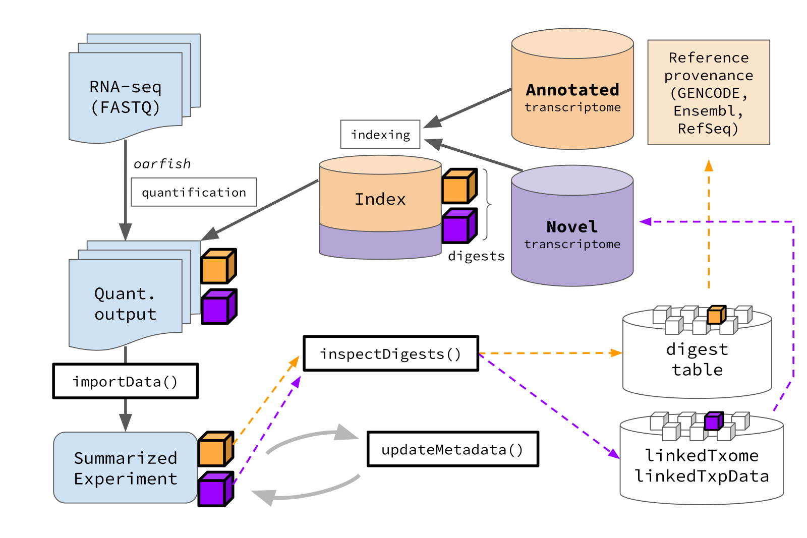
Here we introduce a new workflow for importing data and linking quantification data to metadata, designed for this mixed reference transcript situation, but which may be generalized in the future for other transcript quantification settings.
-
importData()- imports data as an un-ranged SummarizedExperiment -
inspectDigests()- inspects the digest status of the indices for imported data -
updateMetadata()- assists in attaching metadata from matching reference transcriptomes - and linkedTxpData, a lightweight version of linkedTxome, described below
Below is an un-evaluated code chunk with typical code you may use for
an experiment called experiment with samples
rep1 to rep4:
# specify oarfish .quant files
# quantified against an index of two .fa files, e.g.:
# `--annotated gencode.v48.transcripts.fa.gz --novel my_novel_txps.fa.gz`
names <- paste0("rep", 1:4)
files <- file.path(dir, paste0("experiment_", names, ".quant.gz"))
coldata <- data.frame(files, names) # the sample info table
se <- importData(coldata, type="oarfish")
salmon mixed reference
salmon does not record per-sub-index digests natively. To
enable the same mixed reference workflow, a companion Snakemake rule
runs compute_fasta_digest
on the annotated and novel FASTAs at index time and writes a
mixed_ref_digests.json file into each quantification output
directory alongside quant.sf. The Snakemake rules and
further details are available at thelovelab/salmon-with-mixed-ref.
Pass the digest filename to importData() via the
mixedDigest argument:
# specify salmon quant.sf files, quantified against a combined annotated + novel index
names <- paste0("rep", 1:4)
files <- file.path(dir, paste0("experiment_", names, "/quant.sf"))
coldata <- data.frame(files, names)
se <- importData(coldata, type="salmon", mixedDigest="mixed_ref_digests.json")
The returned object and all subsequent steps
(inspectDigests(), updateMetadata()) are
identical to the oarfish workflow described below.
Importing oarfish data
Below is an evaluated code chunk which first points to the location of the dataset used for the vignette. The above code chunk is more typical for a user however.
dir <- system.file("extdata/oarfish", package="tximportData")
names <- paste0("rep", 2:4)
files <- file.path(dir, paste0("sgnex_h9_", names, ".quant.gz"))
coldata <- data.frame(files, names)
# read in the quantification data
se <- importData(coldata, type="oarfish")
## reading in files with read.delim (install 'readr' package for speed up)## 1 2 3
## returning un-ranged SummarizedExperiment, see functions:
## -- inspectDigests() to check matching digests
## -- makeLinkedTxome/makeLinkedTxpData() to link digests to metadata
## -- updateMetadata() to update metadata and optionally add rangesThe importData() function returns an un-ranged
SummarizedExperiment, with no metadata attached. This is similar to what
tximeta() does with skipMeta=TRUE.
class(se)## [1] "SummarizedExperiment"
## attr(,"package")
## [1] "SummarizedExperiment"
rowData(se)## DataFrame with 423044 rows and 0 columnsWe can now inspect the digests of the two indices:
# returns a 2-row tibble
# (here localGENCODE avoids downloading an ftp file)
inspectDigests(se)
## # A tibble: 2 × 8
## index source organism release genome linkedTxome linkedTxpData small_digest
## <chr> <chr> <chr> <chr> <chr> <lgl> <lgl> <chr>
## 1 annotat… Local… Homo sa… 48 GRCh38 TRUE FALSE 6fc626
## 2 novel NA NA NA NA NA NA 43158fWe can see the source and other annotation details for
annotated and for novel. If a match is found
in the pre-computed digests, the linkedTxome digests, or the
linkedTxpData digests, it will populate the
source to genome columns and will indicate if
it is a linkedTxome or linkedTxpData
match.
Note: linkedTxpData is a newly
developed, lightweight version of linkedTxome, which links
quantification data to metadata in the form of a GRanges object
for a set of transcripts. For more details see the man page for
makeLinkedTxpData().
If both linkedTxome and linkedTxpData are
FALSE and the metadata is populated, the digest was a match
among the pre-computed digests.
A small 6-character version of the digest is printed. One can also obtain the full digest (shown below).
inspectDigests(se, fullDigest=TRUE)## # A tibble: 2 × 9
## index source organism release genome linkedTxome linkedTxpData small_digest
## <chr> <chr> <chr> <chr> <chr> <lgl> <lgl> <chr>
## 1 annotat… Local… Homo sa… 48 GRCh38 TRUE FALSE 6fc626
## 2 novel NA NA NA NA NA NA 43158f
## # ℹ 1 more variable: digest <chr>One can also obtain the count (count=TRUE) of matching
transcripts per index, which involves loading transcript data from
locally cached sources (or generating these from local or remote GTF as
needed).
Inspection can be run iteratively, in combination with
makeLinkedTxome() described below or
makeLinkedTxpData(), in order to match up missing digests
with GTF files and/or range-based metadata.
The next step is to run updateMetadata(). This function
does what tximeta() does by default for a single index, by
adding available metadata and attaching to rowData. Thus
updateMetadata() overlaps with previous behavior by
addIds(). Some options here are to add
ranges=TRUE which populates rowRanges but
necessitates removing transcripts (rows) without range information.
Here, transcripts are preserved but NA filled in for
columns where we don’t have metadata.
se_update <- updateMetadata(se)## Warning in .get_cds_IDX(mcols0$type, mcols0$phase): The "phase" metadata column contains non-NA values for features of type
## stop_codon. This information was ignored.## Warning in .makeTxDb_normarg_chrominfo(chrominfo): genome version information
## is not available for this TxDb object## --annotated: adding metadata for 385669 transcripts## --novel: no transcript metadata found
## consider using `linkedTxome`, or `linkedTxpData` (see man pages)## --novel: no matching transcripts
mcols(se_update)## DataFrame with 423044 rows and 4 columns
## tx_name tx_id gene_id index
## <character> <integer> <CharacterList> <character>
## ENST00000832824.1 ENST00000832824.1 1 ENSG00000290825.2 annotated
## ENST00000832825.1 ENST00000832825.1 2 ENSG00000290825.2 annotated
## ENST00000832826.1 ENST00000832826.1 3 ENSG00000290825.2 annotated
## ENST00000832827.1 ENST00000832827.1 4 ENSG00000290825.2 annotated
## ENST00000832828.1 ENST00000832828.1 5 ENSG00000290825.2 annotated
## ... ... ... ... ...
## novel10996 novel10996 NA NA NA
## novel10997 novel10997 NA NA NA
## novel10998 novel10998 NA NA NA
## novel10999 novel10999 NA NA NA
## novel11000 novel11000 NA NA NAupdateMetadata() also allows adding metadata manually,
either in the form of a GRanges object or
data.frame-like object. Note that
makeLinkedTxpData() can be used for persistent addition of
GRanges metadata across sessions.
# define novel set so we can add metadata
novel <- data.frame(
  seqnames = paste0("chr", rep(1:22, each = 500)),
  start = 1e6 + 1 + 0:499 * 1000,
  end = 1e6 + 1 + 0:499 * 1000 + 1000 - 1,
  strand = "+",
  tx_name = paste0("novel", 1:(22 * 500)),
  gene_id = paste0("novel_gene", rep(1:(22 * 10), each = 50)),
  type = "protein_coding"
)
head(novel)
## seqnames start end strand tx_name gene_id type
## 1 chr1 1000001 1001000 + novel1 novel_gene1 protein_coding
## 2 chr1 1001001 1002000 + novel2 novel_gene1 protein_coding
## 3 chr1 1002001 1003000 + novel3 novel_gene1 protein_coding
## 4 chr1 1003001 1004000 + novel4 novel_gene1 protein_coding
## 5 chr1 1004001 1005000 + novel5 novel_gene1 protein_coding
## 6 chr1 1005001 1006000 + novel6 novel_gene1 protein_coding
library(GenomicRanges)
novel_gr <- as(novel, "GRanges")
names(novel_gr) <- novel$tx_name
Metadata specified via the txpData argument will be
added to transcript labelled with index="user".
se_with_ranges <- updateMetadata(se, txpData=novel_gr, ranges=TRUE)## --annotated: adding metadata for 385669 transcripts## --novel: no transcript metadata found
## consider using `linkedTxome`, or `linkedTxpData` (see man pages)## --novel: no matching transcripts## --user: adding metadata for 11000 transcripts## building RangedSE: subsetting to 396669 out of 423044 rows with range data
rowRanges(se_with_ranges)## GRanges object with 396669 ranges and 5 metadata columns:
## seqnames ranges strand | tx_name
## <Rle> <IRanges> <Rle> | <character>
## ENST00000832824.1 chr1 11121-14413 + | ENST00000832824.1
## ENST00000832825.1 chr1 11125-14405 + | ENST00000832825.1
## ENST00000832826.1 chr1 11410-14413 + | ENST00000832826.1
## ENST00000832827.1 chr1 11411-14413 + | ENST00000832827.1
## ENST00000832828.1 chr1 11426-14409 + | ENST00000832828.1
## ... ... ... ... . ...
## novel10996 chr22 1495001-1496000 + | novel10996
## novel10997 chr22 1496001-1497000 + | novel10997
## novel10998 chr22 1497001-1498000 + | novel10998
## novel10999 chr22 1498001-1499000 + | novel10999
## novel11000 chr22 1499001-1500000 + | novel11000
## tx_id gene_id index type
## <integer> <CharacterList> <character> <character>
## ENST00000832824.1 1 ENSG00000290825.2 annotated NA
## ENST00000832825.1 2 ENSG00000290825.2 annotated NA
## ENST00000832826.1 3 ENSG00000290825.2 annotated NA
## ENST00000832827.1 4 ENSG00000290825.2 annotated NA
## ENST00000832828.1 5 ENSG00000290825.2 annotated NA
## ... ... ... ... ...
## novel10996 <NA> novel_gene220 user protein_coding
## novel10997 <NA> novel_gene220 user protein_coding
## novel10998 <NA> novel_gene220 user protein_coding
## novel10999 <NA> novel_gene220 user protein_coding
## novel11000 <NA> novel_gene220 user protein_coding
## -------
## seqinfo: 25 sequences (1 circular) from an unspecified genome; no seqlengthsTwo additional details for inspectDigests() and
updateMetadata():
- The argument
preferspecifies the preferred order of digest match across various tximeta registries. Default istxome: linkedTxome, thentxpdata: linkedTxpData, finallyprecomputed. - One can specify per index, the
key, i.e. the name of the column used for matching metadata. By defaulttx_nameis used.
This new workflow for data import is under active development, feel free to post an Issue with any feedback.
Errors connecting to a database
tximeta makes use of BiocFileCache to store
transcript and other databases, so saving the relevant databases in a
centralized location used by other Bioconductor packages as well. It is
possible that an error can occur in connecting to these databases,
either if the files were accidentally removed from the file system, or
if there was an error generating or writing the database to the cache
location. In each of these cases, it is easy to remove the entry in the
BiocFileCache so that tximeta will know to
regenerate the transcript database or any other missing database.
If you have used the default cache location, then you can obtain access to your BiocFileCache with:
library(BiocFileCache)## Loading required package: dbplyr
bfc <- BiocFileCache()Otherwise, you can recall your particular tximeta cache
location with getTximetaBFC().
You can then inspect the entries in your BiocFileCache using
bfcinfo and remove the entry associated with the missing
database with bfcremove. See the BiocFileCache vignette for
more details on finding and removing entries from a BiocFileCache.
Note that there may be many entries in the BiocFileCache location,
including .sqlite database files and serialized
.rds files. You should only remove the entry associated
with the missing database, e.g. if R gave an error when trying to
connect to the TxDb associated with GENCODE v99 human transcripts, you
should look for the rid of the entry associated with the
human v99 GTF from GENCODE.
What if digest isn’t known?
tximeta automatically imports relevant metadata when the
transcriptome matches a known source – known in the sense that
it is in the set of pre-computed digests in tximeta
(GENCODE, Ensembl, and RefSeq for human and mouse). tximeta
also facilitates the linking of transcriptomes used in building the
salmon index with relevant public sources, in the case that
these are not part of this pre-computed set known to
tximeta. The linking of the transcriptome source with the
quantification files is important in the case that the transcript
sequence no longer matches a known source (uniquely combined or filtered
FASTA files), or if the source is not known to tximeta.
Combinations of coding and non-coding human, mouse, and fruit fly
Ensembl transcripts should be automatically recognized by
tximeta and does not require making a linkedTxome.
As the package is further developed, we plan to roll out support for all
common transcriptomes, from all sources.
Note: if you are using salmon in alignment
mode, then there is no salmon index, and without the salmon index, there
is no digest. We don’t have a perfect solution for this yet, but you can
still summarize transcript counts to gene with a tx2gene
table that you construct manually (see tximport vignette
for example code). Just specify the arguments,
skipMeta=TRUE, txOut=FALSE, tx2gene=tx2gene, when calling
tximeta and it will perform summarization to gene level as
in tximport.
We now demonstrate how to make a linkedTxome and how to share and load a linkedTxome. We point to a salmon quantification file which was quantified against a transcriptome that included the coding and non-coding Drosophila melanogaster transcripts, as well as an artificial transcript of 960 bp (for demonstration purposes only).
dir <- system.file("extdata/salmon_dm", package="tximportData")
file <- file.path(dir, "SRR1197474.plus", "quant.sf")
file.exists(file)
## [1] TRUE
coldata <- data.frame(files=file, names="SRR1197474", sample="1",
                      stringsAsFactors=FALSE)
Trying to import the files gives a message that tximeta
couldn’t find a matching transcriptome, so it returns an non-ranged
SummarizedExperiment.
se <- tximeta(coldata)## importing salmon quantification files## reading in files with read.delim (install 'readr' package for speed up)## 1
## couldn't find matching transcriptome, returning non-ranged SummarizedExperimentLinked transcriptomes
If the transcriptome used to generate the salmon index does not match any transcriptomes from known sources (e.g. from combining or filtering known transcriptome files), there is not much that can be done to automatically populate the metadata during quantification import. However, we can facilitate the following two cases:
- the transcriptome was created locally and has been linked to its public source(s)
- the transcriptome was produced by another group, and they have produced and shared a file that links the transcriptome to public source(s)
tximeta offers functionality to assist reproducible
analysis in both of these cases.
To make this quantification reproducible, we make a
linkedTxome which records key information about the sources
of the transcript FASTA files, and the location of the relevant GTF
file. It also records the digest of the transcriptome that was computed
by salmon during the index step.
Source: when creating the linkedTxome
one must specify the source of the transcriptome. See
?linkedTxome for a note on the implications of this text
string. For canonical GENCODE or Ensembl transcriptomes, one can use
"GENCODE" or "Ensembl", but for modified or
otherwise any transcriptomes defined by a local database, it is
recommended to use a different string, "LocalGENCODE" or
`“LocalEnsembl”, which will avoid tximeta pulling canonical
GENCODE or Ensembl resources from AnnotationHub.
Multiple GTF/GFF files: linkedTxome and
tximeta do not currently support multiple GTF/GFF files,
which is a more complicated case than multiple FASTA, which is
supported. Currently, we recommend that users should add or combine
GTF/GFF files themselves to create a single GTF/GFF file that contains
all features used in quantification, and then upload such a file to
Zenodo, which can then be linked as shown below. Feel free to
contact the developers on the Bioconductor support site or GitHub Issue
page for further details or feature requests.
Stringtie: A special note for building on top of
Stringtie-generated transcripts: it is a good idea to change gene
identifiers, to not include a period ., as the
period will later be used to separate transcript versions from gene
identifiers. This can be done before building the salmon index, by
changing periods in the gene identifier to an underscore. See this GitHub
issue for details.
By default, linkedTxome will write out a JSON file which
can be shared with others, linking the digest of the index with the
other metadata, including FASTA and GTF sources. By default, it will
write out to a file with the same name as the indexDir, but
with a .json extension added. This can be prevented with
write=FALSE, and the file location can be changed with
jsonFile.
First we specify the path where salmon index directory with
indexDir, which will be used to look up the digest and
associate it with the index. Alternatively one can specify the
digest itself and an indexName.
Typically you would not use system.file and
file.path to locate this directory, but simply define
indexDir to be the path of the salmon directory on
your machine. Here we use system.file and
file.path because we have included parts of a
salmon index directory in the tximeta package itself
for demonstration of functionality in this vignette.
indexDir <- file.path(dir, "Dm.BDGP6.22.98.plus_salmon-0.14.1")Now we provide the location of the FASTA files and the GTF file for this transcriptome.
Note: the basename for the GTF file is used as a
unique identifier for the cached versions of the TxDb and the
transcript ranges, which are stored on the user’s behalf via
BiocFileCache. This is not an issue, as GENCODE, Ensembl, and
RefSeq all provide GTF files which are uniquely identified by their
filename,
e.g. Drosophila_melanogaster.BDGP6.22.98.gtf.gz.
The recommended usage of tximeta would be to specify a
remote GTF source, as seen in the commented-out line below:
fastaFTP <- c("ftp://ftp.ensembl.org/pub/release-98/fasta/drosophila_melanogaster/cdna/Drosophila_melanogaster.BDGP6.22.cdna.all.fa.gz",
              "ftp://ftp.ensembl.org/pub/release-98/fasta/drosophila_melanogaster/ncrna/Drosophila_melanogaster.BDGP6.22.ncrna.fa.gz",
              "extra_transcript.fa.gz")
#gtfFTP <- "ftp://path/to/custom/Drosophila_melanogaster.BDGP6.22.98.plus.gtf.gz"
Instead of the above commented-out FTP location for the GTF file, we
specify a location within an R package. This step is just to avoid
downloading from a remote FTP during vignette building. This use of
file.path to point to a file in an R package is specific to
this vignette and should not be used in a typical workflow. The
following GTF file is a modified version of the release 98 from Ensembl,
which includes description of a one transcript, one exon artificial gene
which was inserted into the transcriptome (for demonstration purposes
only).
gtfPath <- file.path(dir,"Drosophila_melanogaster.BDGP6.22.98.plus.gtf.gz")Finally, we create a linkedTxome. In this vignette, we point
to a temporary directory for the JSON file, but a more typical workflow
would write the JSON file to the same location as the salmon
index by not specifying jsonFile.
makeLinkedTxome performs two operation: (1) it creates a
new entry in an internal table that links the transcriptome used in the
salmon index to its sources, and (2) it creates a JSON file
such that this linkedTxome can be shared.
Here we can either specify indexDir or alternatively,
the digest itself and an indexName.
tmp <- tempdir() # just for vignette demo, make temp directory
jsonFile <- file.path(tmp, paste0(basename(indexDir), ".json"))
makeLinkedTxome(indexDir=indexDir,
                source="LocalEnsembl", organism="Drosophila melanogaster",
                release="98", genome="BDGP6.22",
                fasta=fastaFTP, gtf=gtfPath,
                jsonFile=jsonFile)
## reading digest from indexDir: .../Dm.BDGP6.22.98.plus_salmon-0.14.1## writing linkedTxome to /tmp/RtmpjQG2Xe/Dm.BDGP6.22.98.plus_salmon-0.14.1.json## saving linkedTxome in bfcAfter running makeLinkedTxome, the connection between
this salmon index (and its digest) with the sources is saved
for persistent usage. Note that because we added a single transcript of
960bp to the FASTA file used for quantification, tximeta
could tell that this was not quantified against release 98 of the
Ensembl transcripts for Drosophila melanogaster. Only when the
correct set of transcripts were specified does tximeta
recognize and import the correct metadata.
With use of tximeta and a linkedTxome, the
software figures out if the remote GTF has been accessed and compiled
into a TxDb before, and on future calls, it will simply load
the pre-computed metadata and transcript ranges.
Note the warning that 5 of the transcripts are missing from the GTF
file and so are dropped from the final output. This is a problem coming
from the annotation source, and not easily avoided by
tximeta.
se <- tximeta(coldata)## importing salmon quantification files## reading in files with read.delim (install 'readr' package for speed up)## 1
## found matching linkedTxome:
## [ LocalEnsembl - Drosophila melanogaster - release 98 ]
## building TxDb with 'txdbmaker' package
## Import genomic features from the file as a GRanges object ... OK
## Prepare the 'metadata' data frame ... OK
## Make the TxDb object ...## Warning in .makeTxDb_normarg_chrominfo(chrominfo): genome version information
## is not available for this TxDb object## OK
## generating transcript ranges## Warning in checkAssays2Txps(assays, txps):
##
## Warning: the annotation is missing some transcripts that were quantified.
## 5 out of 33707 txps were missing from GTF/GFF but were in the indexed FASTA
## (e.g. this can occur with transcripts located on haplotype chromosomes).
## In order to build a ranged SummarizedExperiment, these txps were removed.
## To keep these txps, and to skip adding ranges, use skipMeta=TRUE
##
## Example missing txps: [FBtr0307759, FBtr0084079, FBtr0084080, ...]We can see that the appropriate metadata and transcript ranges are attached.
rowRanges(se)## GRanges object with 33702 ranges and 3 metadata columns:
## seqnames ranges strand | tx_id gene_id
## <Rle> <IRanges> <Rle> | <integer> <CharacterList>
## Newgene 3R 1-960 + | 20219 Newgene
## FBtr0070129 X 656673-657899 + | 28757 FBgn0025637
## FBtr0070126 X 656356-657899 + | 28753 FBgn0025637
## FBtr0070128 X 656673-657899 + | 28756 FBgn0025637
## FBtr0070124 X 656114-657899 + | 28751 FBgn0025637
## ... ... ... ... . ... ...
## FBtr0114299 2R 21325218-21325323 + | 9300 FBgn0086023
## FBtr0113582 3R 5598638-5598777 - | 24475 FBgn0082989
## FBtr0091635 3L 1488906-1489045 + | 13780 FBgn0086670
## FBtr0113599 3L 261803-261953 - | 16973 FBgn0083014
## FBtr0113600 3L 831870-832008 - | 17070 FBgn0083057
## tx_name
## <character>
## Newgene Newgene
## FBtr0070129 FBtr0070129
## FBtr0070126 FBtr0070126
## FBtr0070128 FBtr0070128
## FBtr0070124 FBtr0070124
## ... ...
## FBtr0114299 FBtr0114299
## FBtr0113582 FBtr0113582
## FBtr0091635 FBtr0091635
## FBtr0113599 FBtr0113599
## FBtr0113600 FBtr0113600
## -------
## seqinfo: 25 sequences from an unspecified genome; no seqlengths
seqinfo(se)## Seqinfo object with 25 sequences from an unspecified genome; no seqlengths:
## seqnames seqlengths isCircular genome
## 2L <NA> <NA> <NA>
## 2R <NA> <NA> <NA>
## 3L <NA> <NA> <NA>
## 3R <NA> <NA> <NA>
## 4 <NA> <NA> <NA>
## ... ... ... ...
## 211000022280481 <NA> <NA> <NA>
## 211000022280494 <NA> <NA> <NA>
## 211000022280703 <NA> <NA> <NA>
## mitochondrion_genome <NA> <NA> <NA>
## rDNA <NA> <NA> <NA>Clear linkedTxomes
The following code removes the entire table with information about the linkedTxomes. This is just for demonstration, so that we can show how to load a JSON file below.
Note: Running this code will clear any information about linkedTxomes. Don’t run this unless you really want to clear this table!
library(BiocFileCache)
if (interactive()) {
  bfcloc <- getTximetaBFC()
} else {
  bfcloc <- tempdir()
}
bfc <- BiocFileCache(bfcloc)
bfcinfo(bfc)
## # A tibble: 9 × 10
## rid rname create_time access_time rpath rtype fpath last_modified_time etag
## <chr> <chr> <chr> <chr> <chr> <chr> <chr> <dbl> <chr>
## 1 BFC1 link… 2026-07-08… 2026-07-08… /tmp… rela… 13bf… NA NA
## 2 BFC2 Dros… 2026-07-08… 2026-07-08… /tmp… rela… 13bf… NA NA
## 3 BFC3 txpR… 2026-07-08… 2026-07-08… /tmp… rela… 13bf… NA NA
## 4 BFC4 exon… 2026-07-08… 2026-07-08… /tmp… rela… 13bf… NA NA
## 5 BFC5 gene… 2026-07-08… 2026-07-08… /tmp… rela… 13bf… NA NA
## 6 BFC6 genc… 2026-07-08… 2026-07-08… /tmp… rela… 13bf… NA NA
## 7 BFC7 txpR… 2026-07-08… 2026-07-08… /tmp… rela… 13bf… NA NA
## 8 BFC8 Dros… 2026-07-08… 2026-07-08… /tmp… rela… 13bf… NA NA
## 9 BFC9 txpR… 2026-07-08… 2026-07-08… /tmp… rela… 13bf… NA NA
## # ℹ 1 more variable: expires <dbl>
# only run the next line if you want to remove your linkedTxome table!
bfcremove(bfc, bfcquery(bfc, "linkedTxomeTbl")$rid)
bfcinfo(bfc)
## # A tibble: 8 × 10
## rid rname create_time access_time rpath rtype fpath last_modified_time etag
## <chr> <chr> <chr> <chr> <chr> <chr> <chr> <dbl> <chr>
## 1 BFC2 Dros… 2026-07-08… 2026-07-08… /tmp… rela… 13bf… NA NA
## 2 BFC3 txpR… 2026-07-08… 2026-07-08… /tmp… rela… 13bf… NA NA
## 3 BFC4 exon… 2026-07-08… 2026-07-08… /tmp… rela… 13bf… NA NA
## 4 BFC5 gene… 2026-07-08… 2026-07-08… /tmp… rela… 13bf… NA NA
## 5 BFC6 genc… 2026-07-08… 2026-07-08… /tmp… rela… 13bf… NA NA
## 6 BFC7 txpR… 2026-07-08… 2026-07-08… /tmp… rela… 13bf… NA NA
## 7 BFC8 Dros… 2026-07-08… 2026-07-08… /tmp… rela… 13bf… NA NA
## 8 BFC9 txpR… 2026-07-08… 2026-07-08… /tmp… rela… 13bf… NA NA
## # ℹ 1 more variable: expires <dbl>Loading linkedTxome JSON files
If a collaborator or the Suppmentary Files for a publication shares a
linkedTxome JSON file, we can likewise use
tximeta to automatically assemble the relevant metadata and
transcript ranges. This implies that the other person has used
tximeta with the function makeLinkedTxome
demonstrated above, pointing to their salmon index and to the
FASTA and GTF source(s).
We point to the JSON file and use loadLinkedTxome and
then the relevant metadata is saved for persistent usage. In this case,
we saved the JSON file in a temporary directory.
jsonFile <- file.path(tmp, paste0(basename(indexDir), ".json"))
loadLinkedTxome(jsonFile)
## saving linkedTxome in bfc (first time)Again, using tximeta figures out whether it needs to
access the remote GTF or not, and assembles the appropriate object on
the user’s behalf.
se <- tximeta(coldata)## importing salmon quantification files## reading in files with read.delim (install 'readr' package for speed up)## 1
## found matching linkedTxome:
## [ LocalEnsembl - Drosophila melanogaster - release 98 ]
## loading existing TxDb created: 2026-07-08 20:48:28
## loading existing transcript ranges created: 2026-07-08 20:48:28## Warning in checkAssays2Txps(assays, txps):
##
## Warning: the annotation is missing some transcripts that were quantified.
## 5 out of 33707 txps were missing from GTF/GFF but were in the indexed FASTA
## (e.g. this can occur with transcripts located on haplotype chromosomes).
## In order to build a ranged SummarizedExperiment, these txps were removed.
## To keep these txps, and to skip adding ranges, use skipMeta=TRUE
##
## Example missing txps: [FBtr0307759, FBtr0084079, FBtr0084080, ...]Clear linkedTxomes again
Finally, we clear the linkedTxomes table again so that the above examples will work. This is just for the vignette code and not part of a typical workflow.
Note: Running this code will clear any information about linkedTxomes. Don’t run this unless you really want to clear this table!
if (interactive()) {
  bfcloc <- getTximetaBFC()
} else {
  bfcloc <- tempdir()
}
bfc <- BiocFileCache(bfcloc)
bfcinfo(bfc)
## # A tibble: 9 × 10
## rid rname create_time access_time rpath rtype fpath last_modified_time etag
## <chr> <chr> <chr> <chr> <chr> <chr> <chr> <dbl> <chr>
## 1 BFC2 Dros… 2026-07-08… 2026-07-08… /tmp… rela… 13bf… NA NA
## 2 BFC3 txpR… 2026-07-08… 2026-07-08… /tmp… rela… 13bf… NA NA
## 3 BFC4 exon… 2026-07-08… 2026-07-08… /tmp… rela… 13bf… NA NA
## 4 BFC5 gene… 2026-07-08… 2026-07-08… /tmp… rela… 13bf… NA NA
## 5 BFC6 genc… 2026-07-08… 2026-07-08… /tmp… rela… 13bf… NA NA
## 6 BFC7 txpR… 2026-07-08… 2026-07-08… /tmp… rela… 13bf… NA NA
## 7 BFC8 Dros… 2026-07-08… 2026-07-08… /tmp… rela… 13bf… NA NA
## 8 BFC9 txpR… 2026-07-08… 2026-07-08… /tmp… rela… 13bf… NA NA
## 9 BFC10 link… 2026-07-08… 2026-07-08… /tmp… rela… 13bf… NA NA
## # ℹ 1 more variable: expires <dbl>
# only run the next line if you want to remove your linkedTxome table!
bfcremove(bfc, bfcquery(bfc, "linkedTxomeTbl")$rid)
bfcinfo(bfc)
## # A tibble: 8 × 10
## rid rname create_time access_time rpath rtype fpath last_modified_time etag
## <chr> <chr> <chr> <chr> <chr> <chr> <chr> <dbl> <chr>
## 1 BFC2 Dros… 2026-07-08… 2026-07-08… /tmp… rela… 13bf… NA NA
## 2 BFC3 txpR… 2026-07-08… 2026-07-08… /tmp… rela… 13bf… NA NA
## 3 BFC4 exon… 2026-07-08… 2026-07-08… /tmp… rela… 13bf… NA NA
## 4 BFC5 gene… 2026-07-08… 2026-07-08… /tmp… rela… 13bf… NA NA
## 5 BFC6 genc… 2026-07-08… 2026-07-08… /tmp… rela… 13bf… NA NA
## 6 BFC7 txpR… 2026-07-08… 2026-07-08… /tmp… rela… 13bf… NA NA
## 7 BFC8 Dros… 2026-07-08… 2026-07-08… /tmp… rela… 13bf… NA NA
## 8 BFC9 txpR… 2026-07-08… 2026-07-08… /tmp… rela… 13bf… NA NA
## # ℹ 1 more variable: expires <dbl>alevin details
For alevin quantification, one should point to the
quants_mat.gz file that contains the counts for all of the
cells. In order to tximeta() to work with alevin
quantification, it requires that alevin was run using gene IDs
in the tgMap step and not gene symbols.
Other quantifiers
tximeta can import the output from any quantifiers that
are supported by tximport, and if these are not
salmon, alevin, or Sailfish output, it will
simply return a non-ranged SummarizedExperiment by default.
An alternative solution is to wrap other quantifiers in workflows
that include metadata information JSON files along with each
quantification file. One can place these files in
aux_info/meta_info.json or any relative location specified
by customMetaInfo, for example
customMetaInfo="meta_info.json". This JSON file is located
relative to the quantification file and should contain a tag
index_seq_hash with an associated value of the SHA-256 hash
(digest) of the reference transcripts. For computing the hash value of
the reference transcripts, see the FastaDigest python
package. The hash value used by salmon is the SHA-256 hash
value of the reference sequences stripped of the header lines, and
concatenated together with the empty string (so only cDNA sequences
combined without any new line characters). FastaDigest can be
installed with pip install fasta_digest.
Acknowledgments
The development of tximeta has benefited from suggestions from these and other individuals in the community:
- Vincent Carey (hashing concept)
- Lori Shepherd (package development, BiocFileCache)
- Martin Morgan (package development)
- Koen Van den Berge
- Johannes Rainer (integration with ensembldb)
- James Ashmore
- Ben Johnson
- Tim Triche
- Kristoffer Vitting-Seerup
- Gordon Smyth and Pedro Baldoni (edgeR and limma functions and docs)
Session info
## Loading required package: usethis## ─ Session info ───────────────────────────────────────────────────────────────
## setting value
## version R version 4.6.1 (2026-06-24)
## os Ubuntu 24.04.4 LTS
## system x86_64, linux-gnu
## ui X11
## language en
## collate en_US.UTF-8
## ctype en_US.UTF-8
## tz UTC
## date 2026-07-08
## pandoc 3.10 @ /usr/bin/ (via rmarkdown)
## quarto 1.9.38 @ /usr/local/bin/quarto
##
## ─ Packages ───────────────────────────────────────────────────────────────────
## package * version date (UTC) lib source
## abind 1.4-8 2024-09-12 [1] RSPM (R 4.6.0)
## AnnotationDbi * 1.75.0 2026-04-28 [1] Bioconductor 3.24 (R 4.6.0)
## AnnotationFilter 1.37.0 2026-04-28 [1] Bioconductor 3.24 (R 4.6.0)
## AnnotationHub 4.3.2 2026-06-30 [1] Bioconductor 3.24 (R 4.6.1)
## Biobase * 2.73.1 2026-04-29 [1] Bioconductor 3.24 (R 4.6.0)
## BiocBaseUtils 1.15.1 2026-05-10 [1] Bioconductor 3.24 (R 4.6.0)
## BiocFileCache * 3.3.0 2026-04-28 [1] Bioconductor 3.24 (R 4.6.0)
## BiocGenerics * 0.59.10 2026-07-07 [1] Bioconductor 3.24 (R 4.6.1)
## BiocIO 1.23.3 2026-04-29 [1] Bioconductor 3.24 (R 4.6.0)
## BiocManager 1.30.27 2025-11-14 [2] CRAN (R 4.6.1)
## BiocParallel 1.47.0 2026-04-28 [1] Bioconductor 3.24 (R 4.6.0)
## BiocVersion 3.24.0 2026-04-28 [2] Bioconductor 3.24 (R 4.6.1)
## biomaRt 2.69.0 2026-04-28 [1] Bioconductor 3.24 (R 4.6.0)
## Biostrings 2.81.5 2026-07-05 [1] Bioconductor 3.24 (R 4.6.1)
## bit 4.6.0 2025-03-06 [1] RSPM (R 4.6.0)
## bit64 4.8.2 2026-05-19 [1] RSPM (R 4.6.0)
## bitops 1.0-9 2024-10-03 [1] RSPM (R 4.6.0)
## blob 1.3.0 2026-01-14 [1] RSPM (R 4.6.0)
## bslib 0.11.0 2026-05-16 [2] RSPM (R 4.6.0)
## cachem 1.1.0 2024-05-16 [2] RSPM (R 4.6.0)
## cigarillo 1.3.0 2026-04-28 [1] Bioconductor 3.24 (R 4.6.0)
## cli 3.6.6 2026-04-09 [2] RSPM (R 4.6.0)
## codetools 0.2-20 2024-03-31 [3] CRAN (R 4.6.1)
## crayon 1.5.3 2024-06-20 [2] RSPM (R 4.6.0)
## curl 7.1.0 2026-04-22 [2] RSPM (R 4.6.0)
## DBI 1.3.0 2026-02-25 [1] RSPM (R 4.6.0)
## dbplyr * 2.6.0 2026-06-17 [1] RSPM (R 4.6.0)
## DelayedArray 0.39.3 2026-06-01 [1] Bioconductor 3.24 (R 4.6.0)
## desc 1.4.3 2023-12-10 [2] RSPM (R 4.6.0)
## devtools * 2.5.2 2026-04-30 [2] RSPM (R 4.6.0)
## digest 0.6.39 2025-11-19 [2] RSPM (R 4.6.0)
## dplyr 1.2.1 2026-04-03 [1] RSPM (R 4.6.0)
## edgeR * 4.11.4 2026-06-28 [1] Bioconductor 3.24 (R 4.6.1)
## ellipsis 0.3.3 2026-04-04 [2] RSPM (R 4.6.0)
## ensembldb 2.37.3 2026-06-07 [1] Bioconductor 3.24 (R 4.6.0)
## evaluate 1.0.5 2025-08-27 [2] RSPM (R 4.6.0)
## fastmap 1.2.0 2024-05-15 [2] RSPM (R 4.6.0)
## filelock 1.0.3 2023-12-11 [1] RSPM (R 4.6.0)
## fs 2.1.0 2026-04-18 [2] RSPM (R 4.6.0)
## generics * 0.1.4 2025-05-09 [1] RSPM (R 4.6.0)
## GenomeInfoDb 1.49.1 2026-05-24 [1] Bioconductor 3.24 (R 4.6.0)
## GenomicAlignments 1.49.0 2026-04-28 [1] Bioconductor 3.24 (R 4.6.0)
## GenomicFeatures * 1.65.0 2026-04-28 [1] Bioconductor 3.24 (R 4.6.0)
## GenomicRanges * 1.65.0 2026-04-28 [1] Bioconductor 3.24 (R 4.6.0)
## glue 1.8.1 2026-04-17 [2] RSPM (R 4.6.0)
## hms 1.1.4 2025-10-17 [1] RSPM (R 4.6.0)
## htmltools 0.5.9 2025-12-04 [2] RSPM (R 4.6.0)
## htmlwidgets 1.6.4 2023-12-06 [2] RSPM (R 4.6.0)
## httr 1.4.8 2026-02-13 [1] RSPM (R 4.6.0)
## httr2 1.2.3 2026-06-23 [2] RSPM (R 4.6.0)
## IRanges * 2.47.2 2026-06-01 [1] Bioconductor 3.24 (R 4.6.0)
## jquerylib 0.1.4 2021-04-26 [2] RSPM (R 4.6.0)
## jsonlite 2.0.0 2025-03-27 [2] RSPM (R 4.6.0)
## KEGGREST 1.53.1 2026-06-16 [1] Bioconductor 3.24 (R 4.6.0)
## knitr 1.51 2025-12-20 [2] RSPM (R 4.6.0)
## lattice 0.22-9 2026-02-09 [3] CRAN (R 4.6.1)
## lazyeval 0.2.3 2026-04-04 [1] RSPM (R 4.6.0)
## lifecycle 1.0.5 2026-01-08 [2] RSPM (R 4.6.0)
## limma * 3.69.2 2026-06-01 [1] Bioconductor 3.24 (R 4.6.0)
## locfit 1.5-9.12 2025-03-05 [1] RSPM (R 4.6.0)
## magrittr 2.0.5 2026-04-04 [2] RSPM (R 4.6.0)
## Matrix 1.7-5 2026-03-21 [3] CRAN (R 4.6.1)
## MatrixGenerics * 1.25.0 2026-04-28 [1] Bioconductor 3.24 (R 4.6.0)
## matrixStats * 1.5.0 2025-01-07 [1] RSPM (R 4.6.0)
## memoise 2.0.1 2021-11-26 [2] RSPM (R 4.6.0)
## org.Dm.eg.db * 3.22.0 2026-06-22 [1] Bioconductor
## otel 0.2.0 2025-08-29 [2] RSPM (R 4.6.0)
## pillar 1.11.1 2025-09-17 [2] RSPM (R 4.6.0)
## pkgbuild 1.4.8 2025-05-26 [2] RSPM (R 4.6.0)
## pkgconfig 2.0.3 2019-09-22 [2] RSPM (R 4.6.0)
## pkgdown 2.2.1.9000 2026-07-08 [1] Github (r-lib/pkgdown@2ee8018)
## pkgload 1.5.3 2026-06-15 [2] RSPM (R 4.6.0)
## png 0.1-9 2026-03-15 [1] RSPM (R 4.6.0)
## prettyunits 1.2.0 2023-09-24 [2] RSPM (R 4.6.0)
## progress 1.2.3 2023-12-06 [1] RSPM (R 4.6.0)
## ProtGenerics 1.45.0 2026-04-28 [1] Bioconductor 3.24 (R 4.6.0)
## purrr 1.2.2 2026-04-10 [2] RSPM (R 4.6.0)
## R6 2.6.1 2025-02-15 [2] RSPM (R 4.6.0)
## ragg 1.5.2 2026-03-23 [2] RSPM (R 4.6.0)
## rappdirs 0.3.4 2026-01-17 [2] RSPM (R 4.6.0)
## RCurl 1.98-1.19 2026-06-03 [1] RSPM (R 4.6.0)
## restfulr 0.0.17 2026-06-11 [1] RSPM (R 4.6.0)
## rjson 0.2.23 2024-09-16 [1] RSPM (R 4.6.0)
## rlang 1.3.0 2026-07-05 [2] RSPM (R 4.6.0)
## rmarkdown 2.31 2026-03-26 [2] RSPM (R 4.6.0)
## Rsamtools 2.29.0 2026-04-28 [1] Bioconductor 3.24 (R 4.6.0)
## RSQLite 3.53.3 2026-06-30 [1] RSPM (R 4.6.0)
## rtracklayer 1.73.0 2026-04-28 [1] Bioconductor 3.24 (R 4.6.0)
## S4Arrays 1.13.0 2026-04-28 [1] Bioconductor 3.24 (R 4.6.0)
## S4Vectors * 0.51.5 2026-06-29 [1] Bioconductor 3.24 (R 4.6.1)
## sass 0.4.10 2025-04-11 [2] RSPM (R 4.6.0)
## Seqinfo * 1.3.0 2026-04-28 [1] Bioconductor 3.24 (R 4.6.0)
## sessioninfo 1.2.4 2026-06-04 [2] RSPM (R 4.6.0)
## SparseArray 1.13.2 2026-05-01 [1] Bioconductor 3.24 (R 4.6.0)
## statmod 1.5.2 2026-05-17 [1] RSPM (R 4.6.0)
## stringi 1.8.7 2025-03-27 [2] RSPM (R 4.6.0)
## stringr 1.6.0 2025-11-04 [1] RSPM (R 4.6.0)
## SummarizedExperiment * 1.43.0 2026-04-28 [1] Bioconductor 3.24 (R 4.6.0)
## systemfonts 1.3.2 2026-03-05 [2] RSPM (R 4.6.0)
## textshaping 1.0.5 2026-03-06 [2] RSPM (R 4.6.0)
## tibble 3.3.1 2026-01-11 [2] RSPM (R 4.6.0)
## tidyselect 1.2.1 2024-03-11 [1] RSPM (R 4.6.0)
## txdbmaker 1.9.0 2026-04-28 [1] Bioconductor 3.24 (R 4.6.0)
## tximeta * 1.31.6 2026-07-08 [1] Bioconductor
## tximport 1.41.0 2026-04-28 [1] Bioconductor 3.24 (R 4.6.0)
## UCSC.utils 1.9.0 2026-04-28 [1] Bioconductor 3.24 (R 4.6.0)
## usethis * 3.2.1 2025-09-06 [2] RSPM (R 4.6.0)
## utf8 1.2.6 2025-06-08 [2] RSPM (R 4.6.0)
## vctrs 0.7.3 2026-04-11 [2] RSPM (R 4.6.0)
## withr 3.0.3 2026-06-19 [2] RSPM (R 4.6.0)
## xfun 0.59 2026-06-19 [2] RSPM (R 4.6.0)
## XML 3.99-0.23 2026-03-20 [1] RSPM (R 4.6.0)
## XVector 0.53.0 2026-04-28 [1] Bioconductor 3.24 (R 4.6.0)
## yaml 2.3.12 2025-12-10 [2] RSPM (R 4.6.0)
##
## [1] /__w/_temp/Library
## [2] /usr/local/lib/R/site-library
## [3] /usr/local/lib/R/library
## * ── Packages attached to the search path.
##
## ──────────────────────────────────────────────────────────────────────────────